Phenotype inference in an Escherichia coli strain panel
Figures
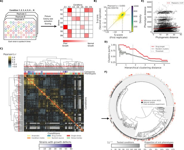
The phenotypic landscape of the E.
coli strain collection. (A) Phenotypic screening experimental design and data analysis. (B) Phenotypic measurements replicability, as measured by pairwise comparing the S-scores of all three biological replicates. (C) Hierarchical clustering of condition correlation profiles; the threshold is defined as the furthest distance at which the minimum average Pearson’s correlation inside each cluster is above 0.3. The two colored bands on top indicate the number of strains with growth defects for each condition and its category, showing consistent clustering. Gray-colored cells in the matrix represent missing values due to poor overlap of strains tested in the two conditions. (D) Clusters purity (computed for drug targets) for each hierarchical distance threshold, against that of random clusters (100 repetitions) shows that drugs with similar target tend to cluster together. (E) Pearson’s correlation between phylogenetic and phenotypic distances, based on phylogenetic independent contrasts (see Materials and methods). (F) Core genome SNP tree for all strains in the collection. Grey shades in the inner ring indicate the number of conditions tested for each strain, red shades in the outer ring indicate the proportion of tested conditions in which the strain shows a significant growth defect. The black arrow indicates the reference strain.
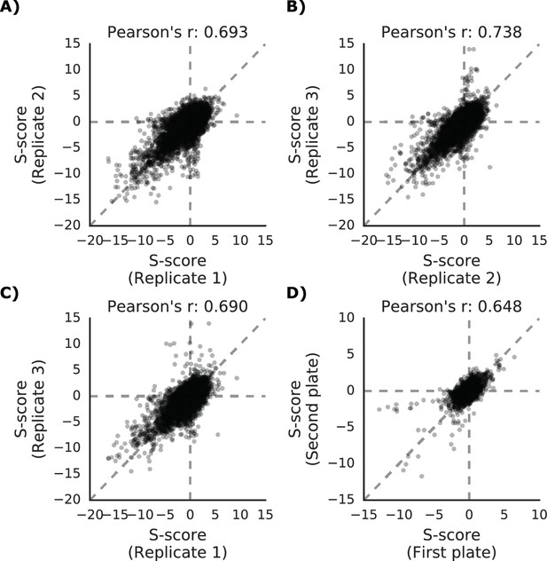
Phenotypic measurements reproducibility and correlation with genetic distance.
(A–C) S-scores for each replicate are compared against each other (D) S-scores comparison between strains present in multiple 1536 plates.
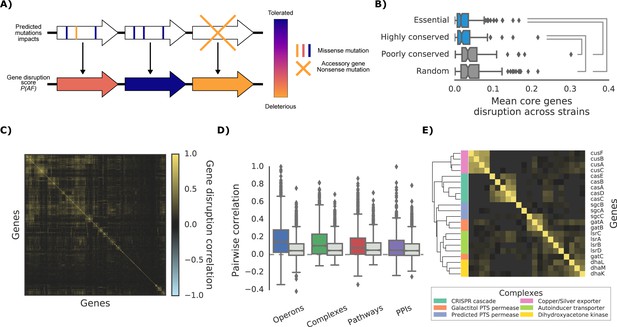
The ‘gene disruption score’, a gene-level prediction of the impact of genetic variants.
(A) Schematic representation of how all substitutions affecting a particular gene are combined to compute the gene disruption score. (B) Average gene disruption score across all strains for four categories of genes conserved in all strains (‘core genome’). Conserved genes are defined as those genes found in more (or less) than 95% of the bacterial species present in the eggNOG orthology database (Huerta-Cepas et al., 2016a). Statistically significant differences (Cohen’s d value >0.3) are reported. (C) Gene-gene correlation profile of gene disruption across all strains shows clusters of potentially functionally related proteins. (D–E) The gene disruption profiles as a predictor of genes function. (D) Pairwise correlation of gene disruption scores inside each annotation set (colored boxes) and inside a random set of genes of the same size (grey boxes). (E) Gene-gene correlation profile of gene disruption scores in protein complexes; shown here a subset with high disruption score correlation.
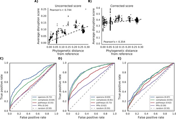
Additional properties of the gene disruption score.
(A) Correlation between phylogenetic distance from the reference strain and average disruption across all reference genes. (B) Significant reduction in correlation after correction of the disruption score (see Materials and methods). (C–E) Prediction of gene functional associations using disruption score profiles. (C) ROC curve using disruption score profiles across all genes. (D–E) Higher predictive power of the gene disruption profile when restricted to accessory genes, including (D) or not (E) the information about gene presence absence.
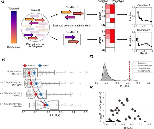
Prediction of growth-defect phenotypes in the E.coli strain collection.
(A) Schematic representation of the computation of the prediction score and its evaluation; for each condition the predicted score is computed using the disruption score of the conditionally essential genes. The score is then evaluated against the actual phenotypes through a Precision-Recall curve. (B) Higher predictive power for conditions with higher proportion of growth phenotypes. For each condition set, the PR-AUC value for each condition is reported, together with the median and mean value (C) Significance of the PR-AUC value reported for the condition ‘Clindamycin 3 μg/ml’, against the distribution of three randomization strategies. ‘Shuffled strains’ indicates a prediction in which the actual strains’ phenotypes have been shuffled; ‘shuffled sets’ indicates a prediction where the conditionally essential genes of a different condition have been used, and ‘random set’ indicates a prediction where a random gene set has been used as conditionally essential genes. For all three randomizations we report a significant difference between the actual prediction and the distribution of the randomizations (q-values of 1E-30, 0.05 and 1E-22, respectively). See Figure 3—figure supplement 2 for the other conditions. (D) Genome-wide gene associations are in agreement with the predictive score; the enrichment of conditionally essential genes in the results of the gene association analysis is significantly higher in conditions with higher PR-AUC.
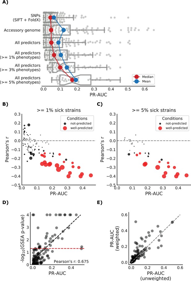
Detailed view of the predicted growth score and its properties.
(A) Influence of the different predictors of the impact of mutations on each condition PR-AUC. ‘SNPs’ indicates single nucleotide variants only, ‘Accessory genome’ gene presence-absence patterns, ‘All predictors’ the combination of both, plus stop codon substitutions. (B–C) Proportion of well-predicted conditions (PR-AUC >= 0.1 and Pearson’s FDR-corrected p-value<=0.01) over total conditions with at least 1% and 5% sick strains. Marker’s size is proportional to the of the FDR-corrected p-value. (E) Conditions with higher predictive power (measured as PR-AUC) also have an enrichment of sick strains at the top of the predicted score, as measured by the Gene Set Enrichment Analysis (GSEA); sick strains are used as ‘gene sets’. A pseudocount of 10−4 has been added to the GSEA p-values. (F) Prediction performance improves when using the weighting scheme to account for conservation of gene essentiality, especially for well-predicted conditions.
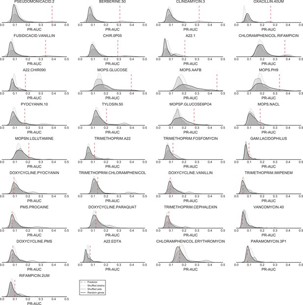
Significance of the PR-AUC value reported for all conditions with at least 5% of the tested strains showing a sick phenotype, against the distribution of three randomization strategies.
‘Shuffled strains’ indicates a prediction in which the actual strains’ phenotypes has been shuffled; ‘shuffled sets’ indicates a prediction where the conditionally essential genes of a different condition have been used, and ‘random set’ indicates a prediction where a random gene set has been used as conditionally essential genes. Conditions are ordered by the significance of the difference between the actual prediction and the ‘Random genes’ bootstrap. The proportion of conditions where the actual prediction is significantly different than the randomizations (q-value <0.05) are 52%, 21% and 33.3% for the ‘shuffled strains’, ‘shuffled sets’ and ‘random genes’ randomizations, respectively.
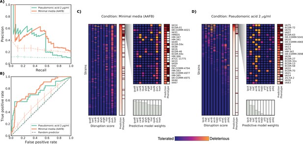
Detailed example on the computation and evaluation of the predicted score on two conditions.
(A) Precision-Recall curve for the two example conditions. Dashed lines represent the average Precision-Recall curve for the same predictions carried out using 10’000 random gene sets of the same size of the actual conditionally essential genes for both conditions. Vertical lines represent the mean absolute deviation for the precision across the randomizations. The two randomization sets are significantly different than the actual predictions (q-values of 1E-33 and 0.02, respectively). (B) Receiver operating characteristic curve for the two example conditions. Dashed lines represent the same randomizations as in (A). (C–D) For each condition, the gene disruption score for the conditionally essential gene across all strains is reported, together with the resulting predicted conditional score and actual binary phenotypes (pale red: healthy and red: growth defect). Strains are sorted according to the predicted conditional score, while genes are sorted according to their weight in the predictive model; only the top 10 conditionally essential genes are shown. The inset reports the disruption score, predicted score and actual phenotypes for the top 25 strains.
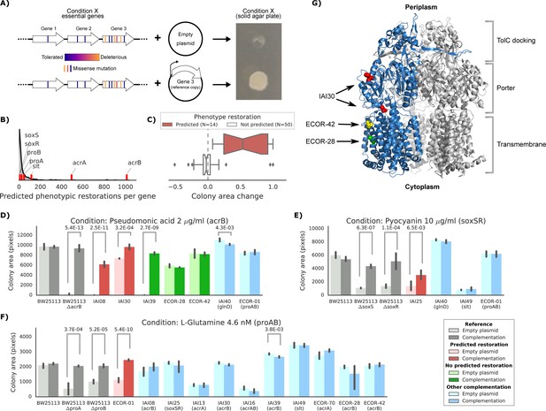
Experimental confirmation of the predicted phenotype-causing genotypes.
(A) Schematic representation of the experimental approach. (B) Distribution of the number of predicted restored phenotypes per gene; red stripes indicate the genes that were experimentally tested. (C) Growth change between the target strain with the empty plasmid against the one expressing the reference copy of the target gene (complementation). Strains for which a change in phenotype is predicted are compared to those where no change is predicted. (D–F) Detailed representation of the results of the complementation experiment in three conditions. Mean colony area and the 95% confidence intervals are reported. Significant differences (t-test p-value<0.01) between colony area of the strains with the empty and complemented plasmids are reported. ‘Other complementation’ reports strains expressing a different gene than the focal one, indicated between parenthesis. (G) Cartoon representation of AcrB 3D structure (PDB entry: 2dr6). Only one of the three monomers is highlighted in blue; colored spheres represent known non-synonymous variants in the reported strains.
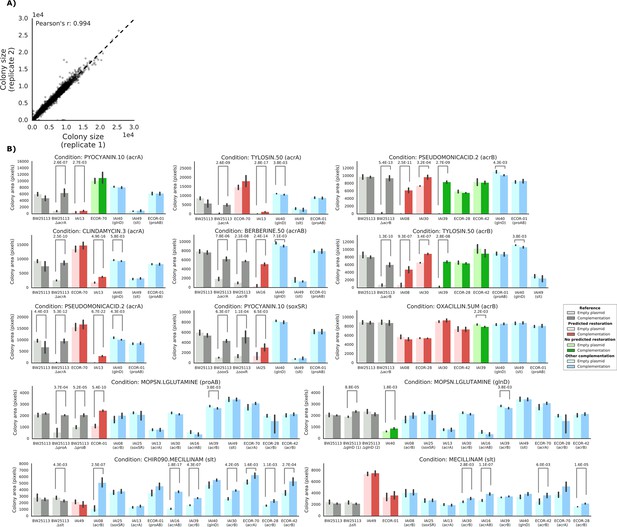
Detailed view of the experimental confirmation of the predicted phenotype-causing genotypes.
(A) Replicability in colony size (measured in pixels) after outer frame and spatial correction between the two replicates. (B) Overview of the results of the complementation experiments. Mean colony area and the 95% confidence intervals are reported. Significant differences (t-test p-value<0.01) between colony area of the strains with the empty and complemented plasmids are reported. Conditions CHIR090.MECILLINAM, MECILLINNAM and OXACILLIN.5UM have been excluded from further analysis, as the deletion strain from the KEIO collection (positive control) does not show a sick phenotype with an empty plasmid.

Additional files
-
Source code 1
code used to analyze the genetic and phenotypic data, predict phenotypes and draw all the manuscript figures.
- https://doi.org/10.7554/eLife.31035.012
-
Supplementary file 1
detailed list of the members of the strain collection
- https://doi.org/10.7554/eLife.31035.013
-
Supplementary file 2
detailed list of conditions on which the strain collection has been tested
- https://doi.org/10.7554/eLife.31035.014
-
Supplementary file 3
categorization and mode of action (MoA) of each chemical used in the phenotypic screening
- https://doi.org/10.7554/eLife.31035.015
-
Supplementary file 4
s-scores, FDR corrected p-values and binary growth defect matrix of the E. coli phenotypic screening (869 strains across 214 conditions)
- https://doi.org/10.7554/eLife.31035.016
-
Supplementary file 5
.disruption scores, conditional scores and prediction assessments.
- https://doi.org/10.7554/eLife.31035.017
-
Transparent reporting form
- https://doi.org/10.7554/eLife.31035.018


