Covert shift of attention modulates the value encoding in the orbitofrontal cortex
- CAS Center for Excellence in Brain Science and Intelligence Technology, Shanghai Institutes for Biological Sciences, Chinese Academy of Sciences, China
- University of Chinese Academy of Sciences, China
Figures
Figure 1
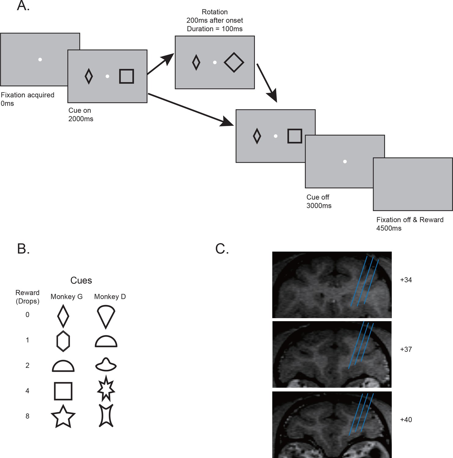
Behavior paradigms and electrophysiology recording locations.
(A) Behavior paradigm. The monkeys had to maintain their fixation while passively viewing one or two visual cues presented on the screen. Each cue was associated with a reward. In some trials, one of the cues was quickly rotated back and forth for 100 ms. At the end of the trial, the monkey received reward associated with one randomly selected cue from the pair. (B) Cue-reward associations used in two monkeys. (C) Estimated recording locations. The structural MRI images shown were from monkey G.
Figure 2 with 3 supplements
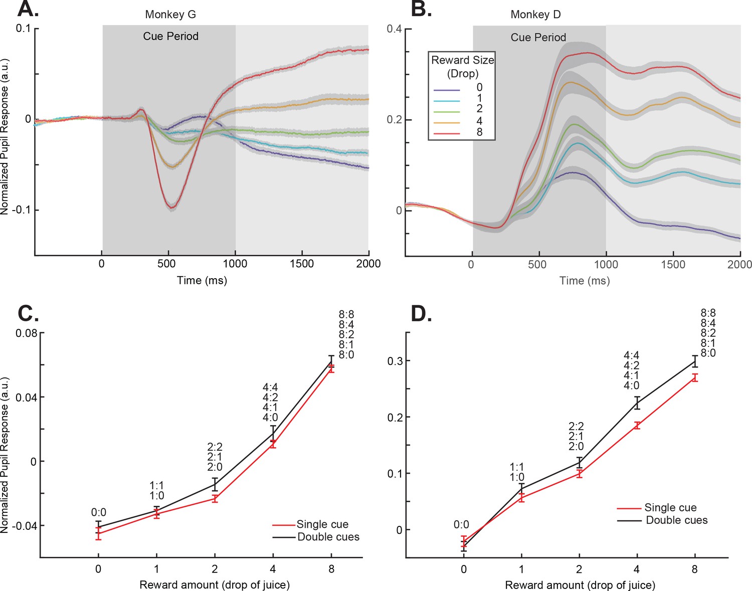
Pupil dilation responses reflected cue-reward association.
(A) Pupil dilation responses of trials in the single-cue conditions for monkey G. Time 0 indicates the cue onset. The dark gray box indicates the cue presentation period. The light gray box indicates the period in which the mean pupil responses were calculated and plotted in panel (C). The colors indicate cues with different rewards. The shading around each curve represents s.e.m. between sessions. (C) Pupil dilation responses of both the single- and double-cue condition trials for monkey G. The responses are calculated as the average pupil size within 1 s after the cue offset, indicated by the light gray box in panel (A). Trials in the double-cue conditions (black curve) are grouped by the higher value between the two cues. The numbers near each data point indicate the cue combinations that comprise each group. The error bars represent s.e.m. between sessions. (B) and (D) Plots for monkey D.
Figure 2—figure supplement 1

Pupil responses for each cue combination.
(A) Pupil responses for each cue combination for monkey G. The cue combinations with the same higher value cue form groups, which are indicated by the same color and joined together by line segments. (B) Pupil responses for monkey D. One-way ANOVAs with Bonferroni corrections were used to test if there are significant differences within each group. See also Supplementary file 1, Table 2.
Figure 2—figure supplement 2

The pupil responses did not reflect the value of the perturbed cue.
The sessions in which value-encoding neurons were recorded are plotted. Time 0 indicates the onset of cues. The blue and red curves are pupil responses when the lower and the higher value cue was rotated. The shading region around the curves represents the s.e.m between sessions. There was no significant difference between the two curves in either monkey.
Figure 2—figure supplement 3
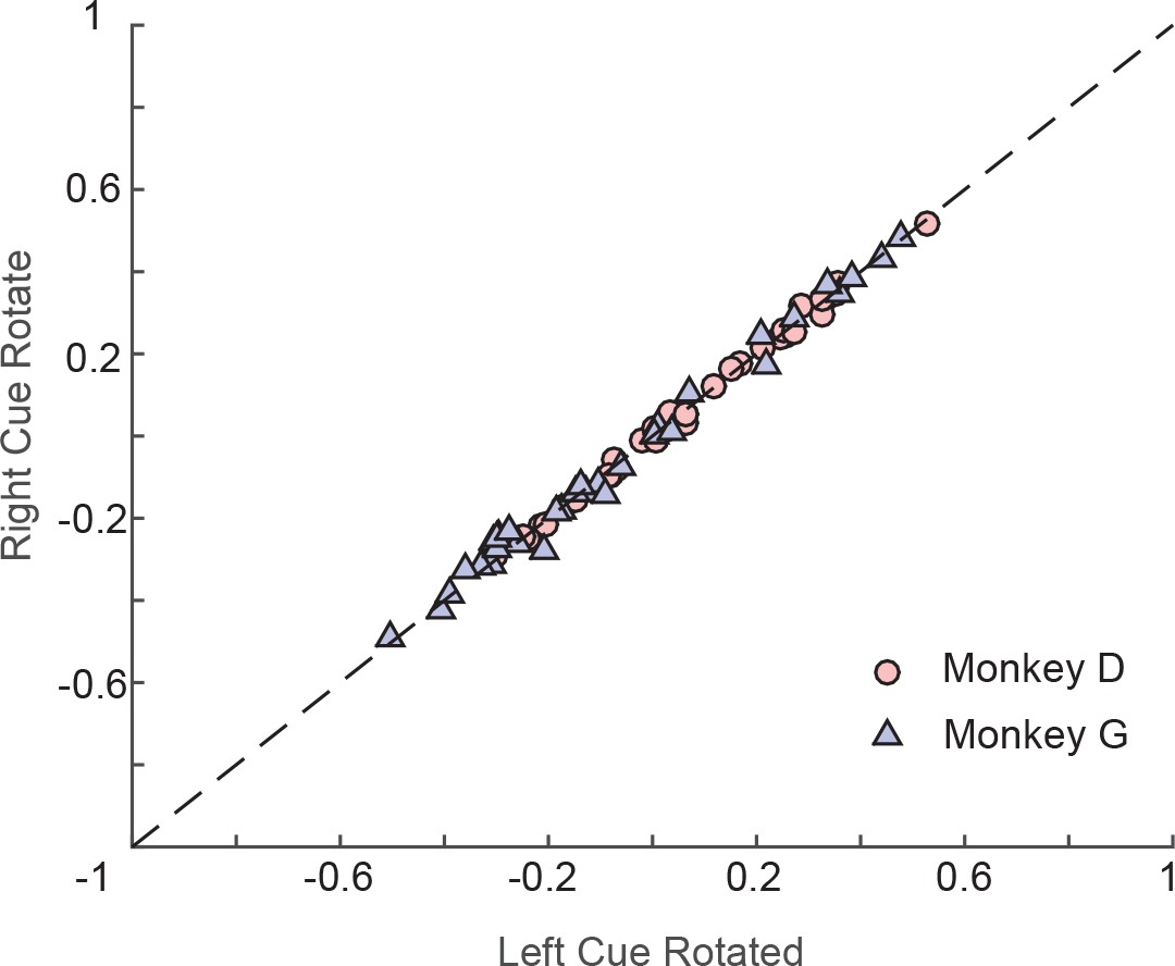
The monkeys’ eye positions during fixation were not affected by visual perturbations.
Each data point represents the average horizontal eye position between the rotation onset and the cue offset under two perturbation locations (left vs. right) in a recording session. The dashed line is the diagonal. The red circles represent monkey D, and the blue triangles represent monkey G. There were no significant shifts away from the diagonal caused by visual perturbations (p=0.4811, two-tailed paired t-test).
Figure 3 with 1 supplement

OFC responses to cue conditions without perturbations.
(A) The PSTH in the single-cue condition of an example OFC neuron. The trials are grouped by the cue’s associated reward value indicated by different colors. The shading around each curve represents s.e.m. between trials. (B) The cue responses to both the single- and double-cue conditions of the example neuron. Trials in the double-cue conditions (black curve) are grouped by the higher value between the two cues. The numbers near each data point indicate the cue combinations that comprise each group. The error bars represent s.e.m. between trials. (C) and (D) The population cue responses to both the single- and double-cue conditions of the positively (C) and the negatively tuned (D) OFC neurons, plotted in a similar format as in panel B. The error bars represent s.e.m. between neurons. (E) The responses of each OFC neuron to both the single- and double-cue conditions. Red and blue data points indicate the positively and the negatively tuned neurons. The red and blue histogram insets are the distributions of response differences between the single- and the double-cue conditions for the positively and the negatively tuned neurons, respectively. Double-cue condition trials are grouped by the higher value.
Figure 3—figure supplement 1
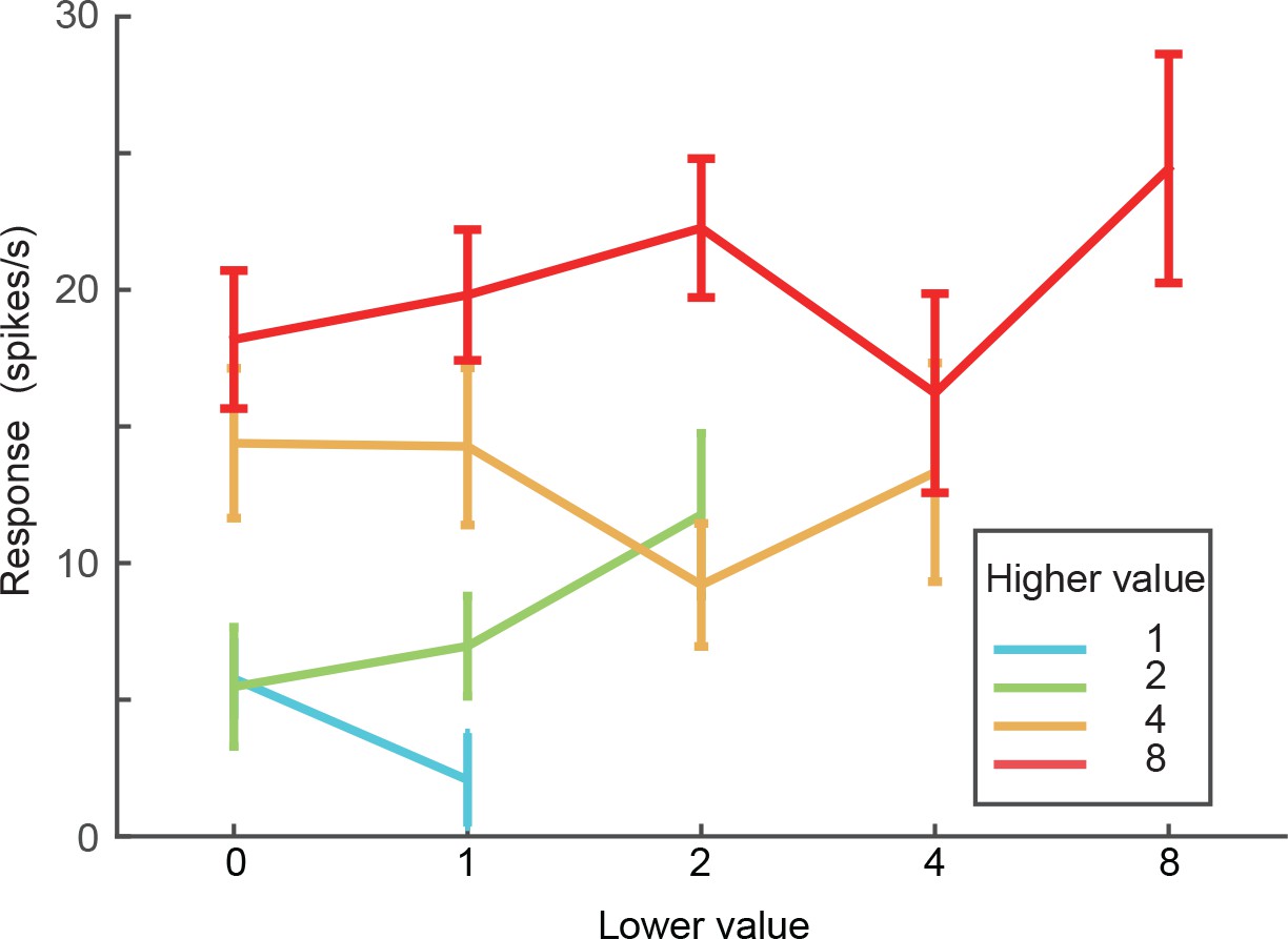
Firing rates of the example neuron in Figure 3AB for each cue combination.
One-way ANOVA showed no significant difference within any of the four groups with the higher value being 1, 2, 4, and 8 (p-values=0.6644, 0.3017, 0.6987, and 0.5031).
Figure 4 with 8 supplements
OFC responses to cue conditions with perturbations.
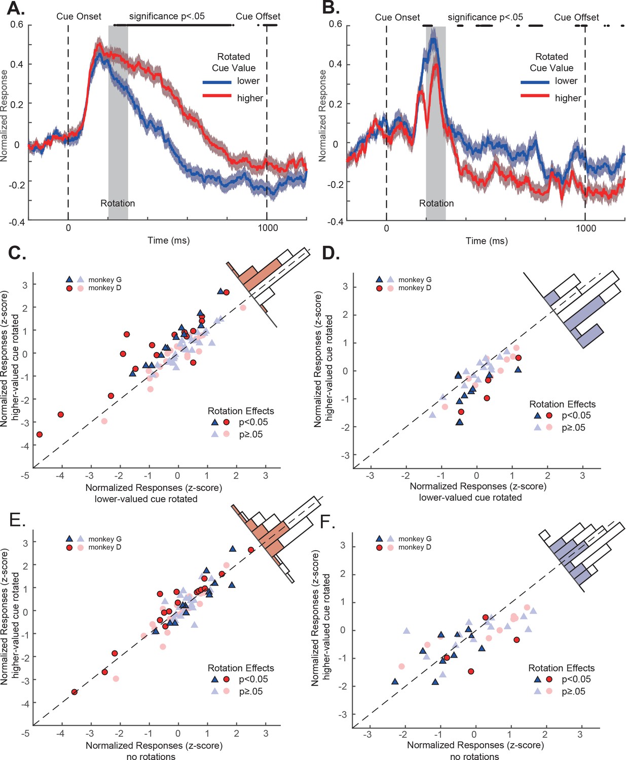
(A) Population responses of the positively tuned OFC neurons to the double-cue conditions with visual perturbations. The blue curve includes the trials with the lower value cue rotated. The red curve includes the trials with the higher value cue rotated. The shading around each curve represents s.e.m. between trials. The grey box indicates the rotation period. The black dots on the top indicates the time points where the difference between two curves is significant (p<0.05 with multiple comparison corrections). (B) Population responses of the negatively tuned OFC neurons to the double-cue conditions with visual perturbations plotted in the same way as in panel A. (C) The comparison between each positively tuned neuron’s responses when the higher and the lower value cues were rotated. Each data point represents a neuron. Bright data points are neurons that showed significant rotation effects, and dim data points are neurons that were not significantly affected by rotations. Blue triangles are neurons from monkey G, and Red circles are from monkey D. A histogram of the response differences between the two conditions is shown on the top right corner, in which filled squares indicate neurons with significant rotation effects. (D) Similar to C, but for the negatively tuned neurons. (E) The comparison between each positively tuned neuron’s responses when the higher value cue was rotated and when there was no perturbation. Bright and dim data points are the same neurons with significant rotation effects as shown in panel (C). The color in the histogram also indicates the same significance as shown in panel C. (F) Similar to (E), but for the negatively tuned neurons.
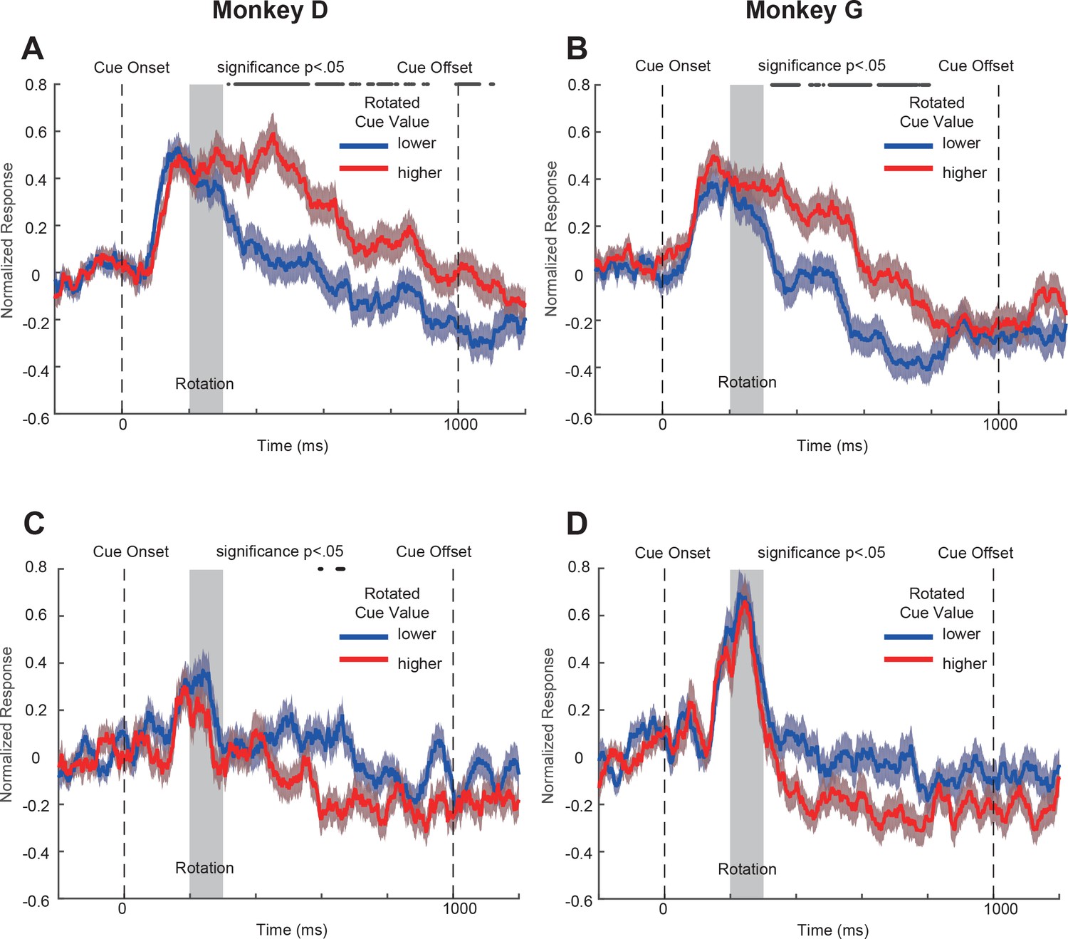
Figure 4—figure supplement 1
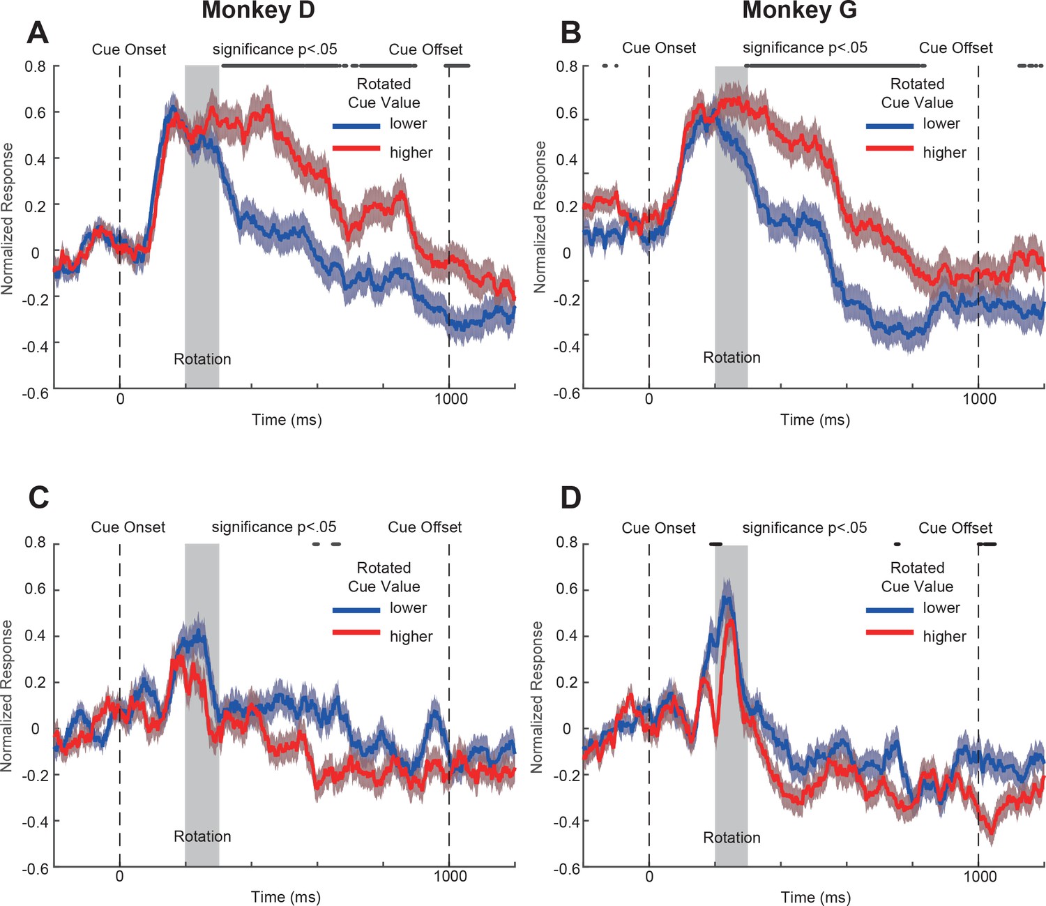
Population responses to the double-cue conditions with visual perturbations of the OFC neurons from individual monkeys.
(A) and (B) Positively tuned neurons from monkeys D and G, respectively. (C) and (D) Negatively tuned neurons from monkeys D and G, respectively. The same convention is used as in Figure 4AB.
Figure 4—figure supplement 2
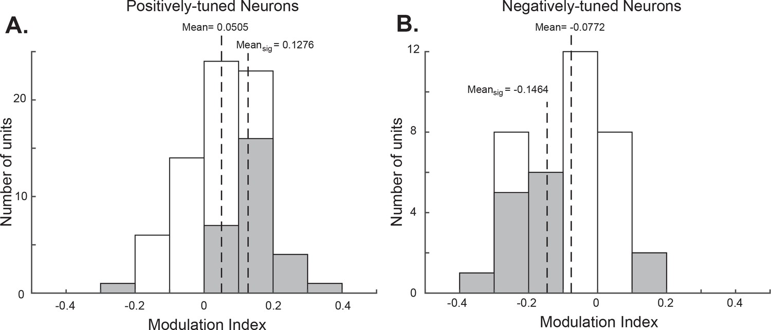
Attentional modulation indices of the value-encoding OFC neurons.
The grey bars indicate neurons with significant attentional modulation. Mean values of all value-encoding neurons and those with significant attentional modulations are indicated by the dashed lines respectively. All of them are significantly different from zero (for all the positively tuned neurons, p=1.10e-4; for the positively tuned neurons with significant attentional modulation, p=4.06e-8, for all the negatively tuned neurons, p=3.04e-4; and for the negatively tuned neurons with significant attentional modulation, p=0.0016).
Figure 4—figure supplement 3
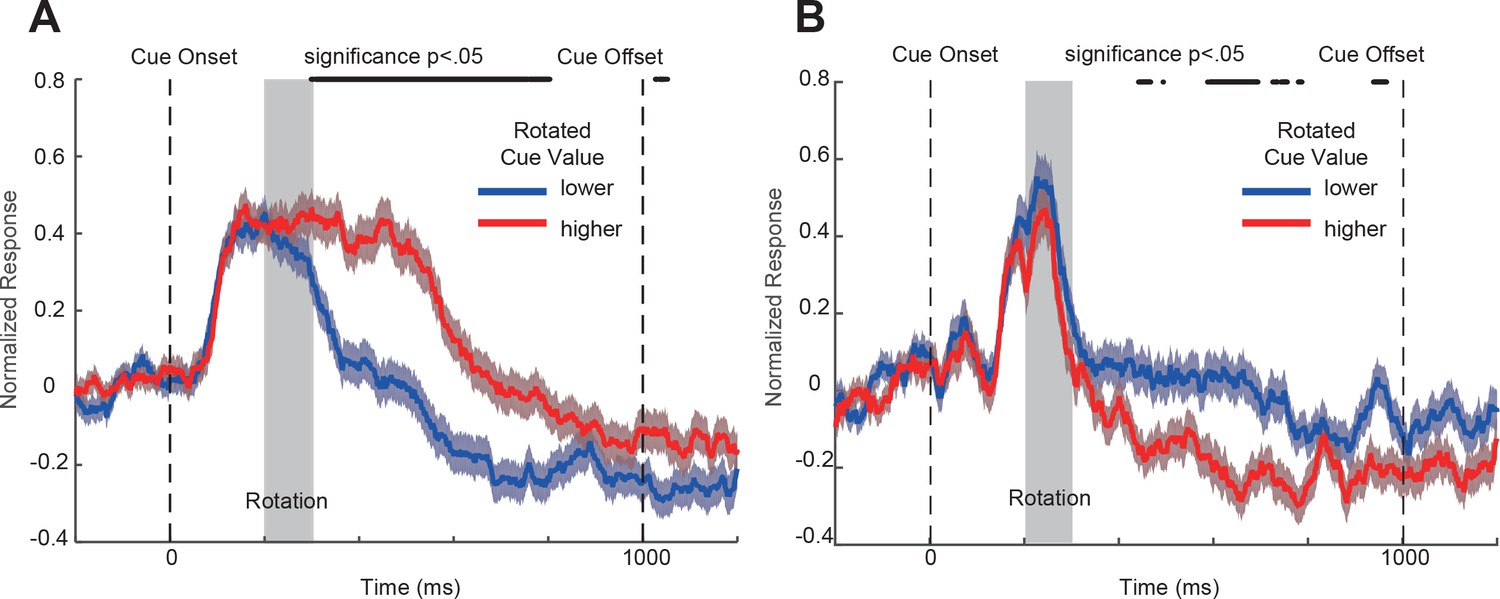
OFC responses to the cue conditions with perturbations.
Analyses are the same as in Figure 4AB, except that only the first 50 correct trials in each block were included. (A) Population responses to the double-cue conditions with visual perturbations of the positively tuned OFC neurons. The blue curve includes the trials with the lower value cue rotated. The red curve includes the trials with the higher value cue rotated. The shading around each curve represents s.e.m. between trials. The grey box indicates the rotation period. The black dots on the top indicates the time points where the difference between two curves is significant (p<0.05 with multiple comparison corrections). (B) Population responses to the double-cue conditions with visual perturbations of the negatively-tuned OFC neurons plotted in the same way as in panel A.
Figure 4—figure supplement 4
Population responses to the double-cue conditions with visual perturbations of the OFC neurons from individual monkeys, with only the first 50 correct trials in each block were included.
(A) and (B) Positively tuned neurons from monkeys D and G, respectively. (C) and (D) Negatively tuned neurons from monkeys D and G, respectively. The same convention is used as in Figure 4AB.
Figure 4—figure supplement 5
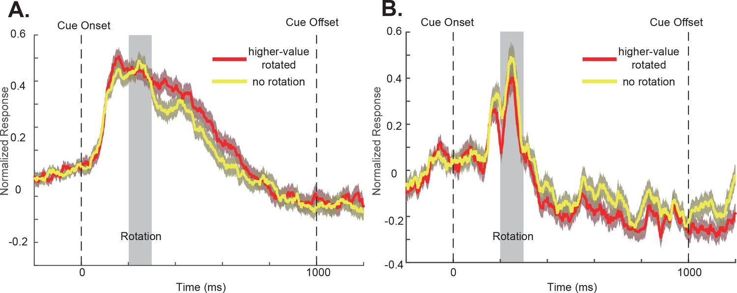
OFC population responses to the double-cue conditions without visual perturbations (yellow) and with visual perturbations applied to the higher value cues (red).
The shading around each curve represents s.e.m. between trials. The grey box indicates the rotation period. Only the neurons with significant attentional modulations were included. (A) The positively tuned OFC neurons. (B) the negatively tuned OFC neurons. No significant differences were found at any time points in either group of neurons (two-tailed t-test with multiple comparisons corrections with the Benjamini-Hochberg procedure with the false discovery rate ≤ 0.05).
Figure 4—figure supplement 6

The history of attentional modulation of OFC responses.
Here, we replotted Figure 4CD, but now labeling the data points by when the neuron was recorded. We split the whole experiment into two halves. The red dots are the sessions in the early half, and the blue ones are in the late half. They largely overlap, indicating that the response difference between the higher value rotated and lower value cue rotated conditions did not differ between the early and the late recording sessions in the study. (Two-tailed t-test. p=0.9244 for the positively tuned neurons; p=0.7898, for the negatively tuned neurons). (A) positively tuned neurons, (B) negatively tuned neurons.
Figure 4—figure supplement 7
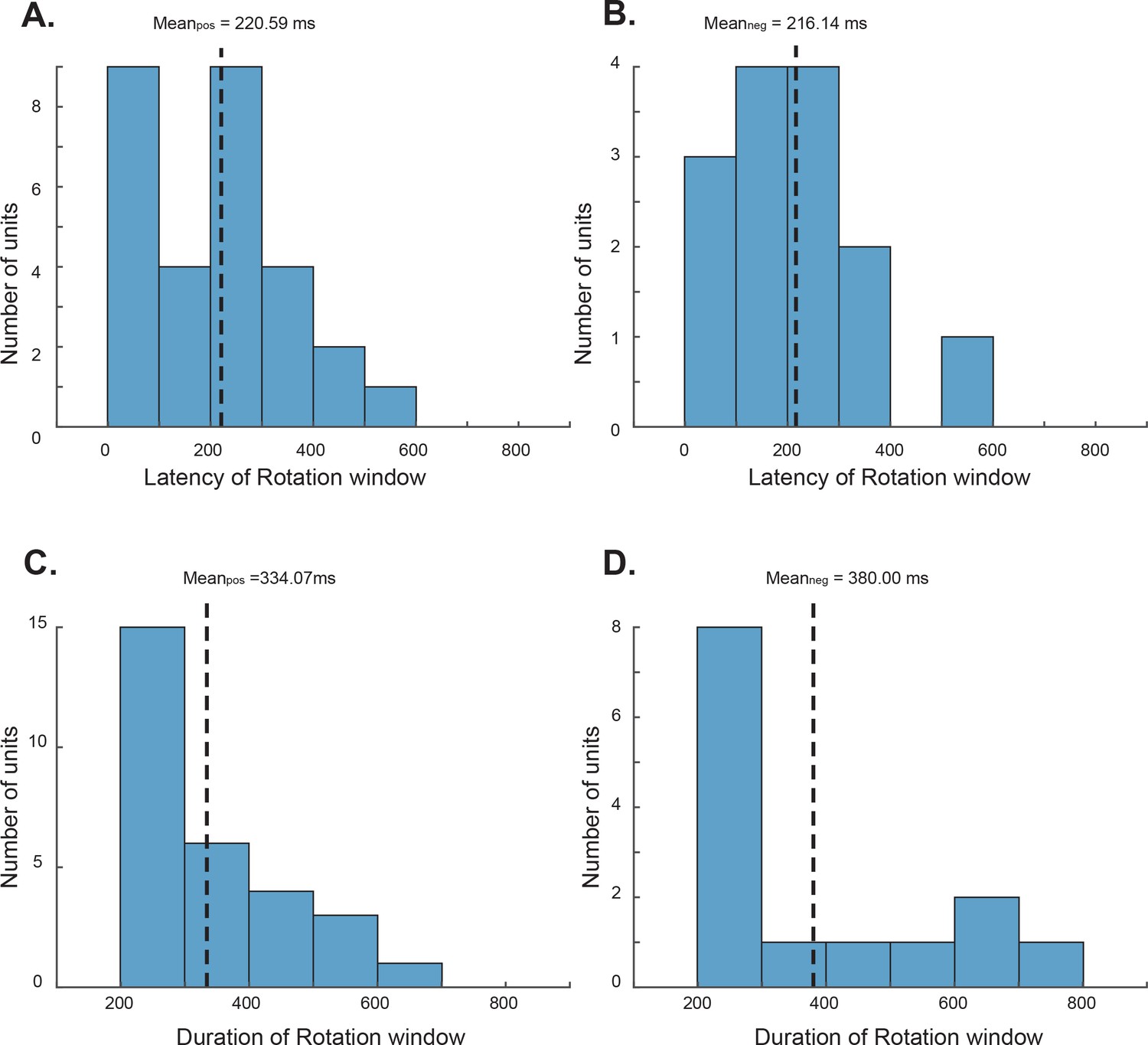
The distributions of the latencies and the durations of the attention modulation window in which the visual perturbation affected the neurons’ responses significantly.
(A) Modulation window latencies for the positively tuned neurons. (B) Modulation window latencies for the negatively tuned neurons. (C) Modulation window durations for the positively tuned neurons. (D) Modulation window durations for the negatively tuned neurons. Mean values are indicated by the dashed lines.
Figure 4—figure supplement 8

OFC neurons’ responses to the double-cue conditions with perturbations applied to the higher value or the lower value cues.
The responses are the average responses from 450 to 750 ms after the cue onset. (A) Positively tuned neurons, (B) negatively tuned neurons. The same convention is used as in Figure 4CD.
Figure 5 with 4 supplements
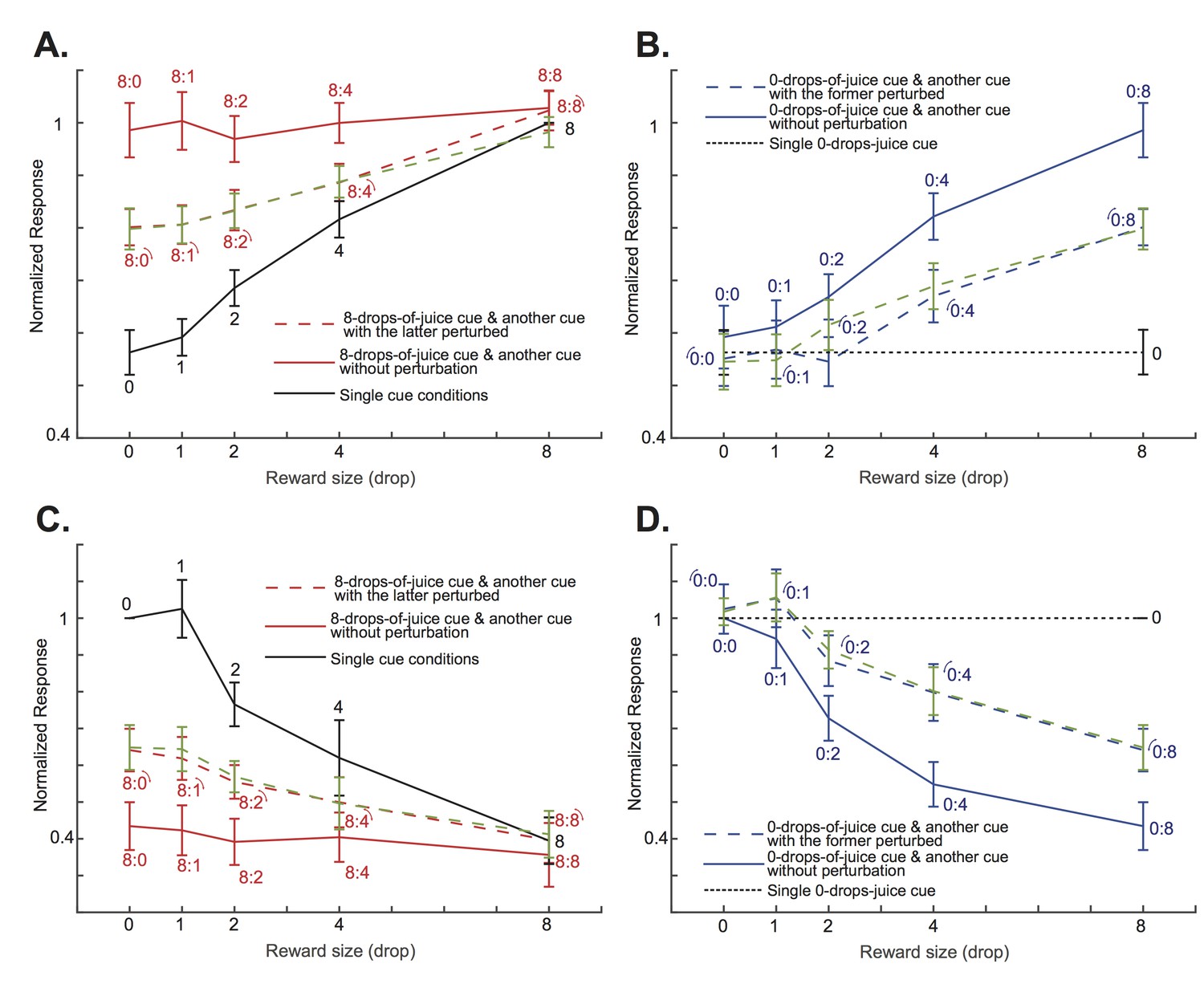
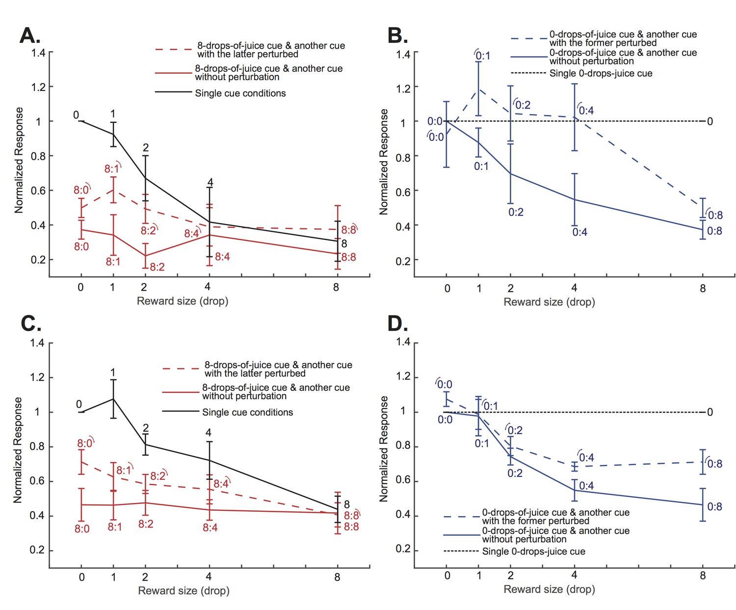
The attentional shift between the two cues depended on the difference between their associated value.
(A) The solid red curve is the positively tuned OFC neurons’ responses to an 8-drops-of-juice cue paired with another cue associated with 0, 1, 2, 4, or 8 drops of juice. The solid black curve indicates the responses to the lower value cue presented alone. The red dashed curve is the responses to the cue pairs with the visual perturbation applied to the lower value cue from the testing data set. The green dashed curve is the predicted responses of the testing dataset by the normalization model fitted with the training dataset. The numbers near each data point indicate the cue combinations that comprise each data point, with the little arcs indicating the perturbed cue. The error bars indicated s.e.m. between neurons. Notice that the responses were normalized to the responses under the neurons’ preferred single-cue condition. Thus, there is no error bar for the 8-drops-of-cue condition. (B) The solid blue curve is the positively tuned OFC neurons’ responses to a 0-drops-of-juice cue paired with another cue associated with 0, 1, 2, 4, or 8 drops of juice. The dotted black horizontal line indicates the responses to the single 0-drops-of-juice cue. The blue dashed line is the responses to the same cue pairs with the visual perturbation applied to the 0-drops-of-juice cue. The green dashed curve is the responses predicted by the normalization model. The numbers near each data point indicate the cue combinations that comprise each data point, with the little arcs indicating the perturbed cue. (C) and (D). The same analyses as panels (A) and (B), but for the negatively-tuned OFC neurons. All error bars indicate s.e.m. between neurons.
Figure 5—figure supplement 1

The modulation of the positively tuned neurons’ responses due to the attentional shift between the two cues depended on the difference between their associated values.
(A) and (C) Similar to Figure 5A, but plotted separately for monkey D and G, respectively. (B) and (D) similar to Figure 5B, but plotted separately for monkey D and G, respectively.
Figure 5—figure supplement 2
The modulation of the negatively tuned neurons’ responses due to the attentional shift between the two cues depended on the difference between their associated values.
(A) and (C) similar to Figure 5C, but plotted separately for monkey D and G, respectively. (B) and (D) similar to Figure 5D, but plotted separately for monkey D and G, respectively.
Figure 5—figure supplement 3
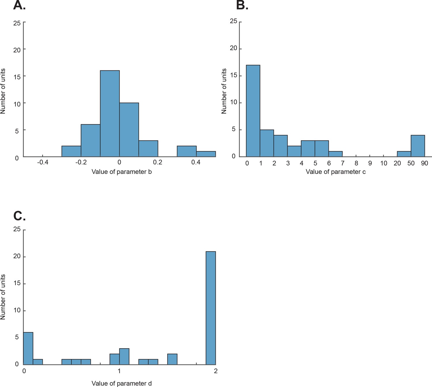
The distributions of the best fitting parameters in the full model of each neuron.
(A) parameter b. (B) parameter c. (C) parameter d.
Figure 5—figure supplement 4
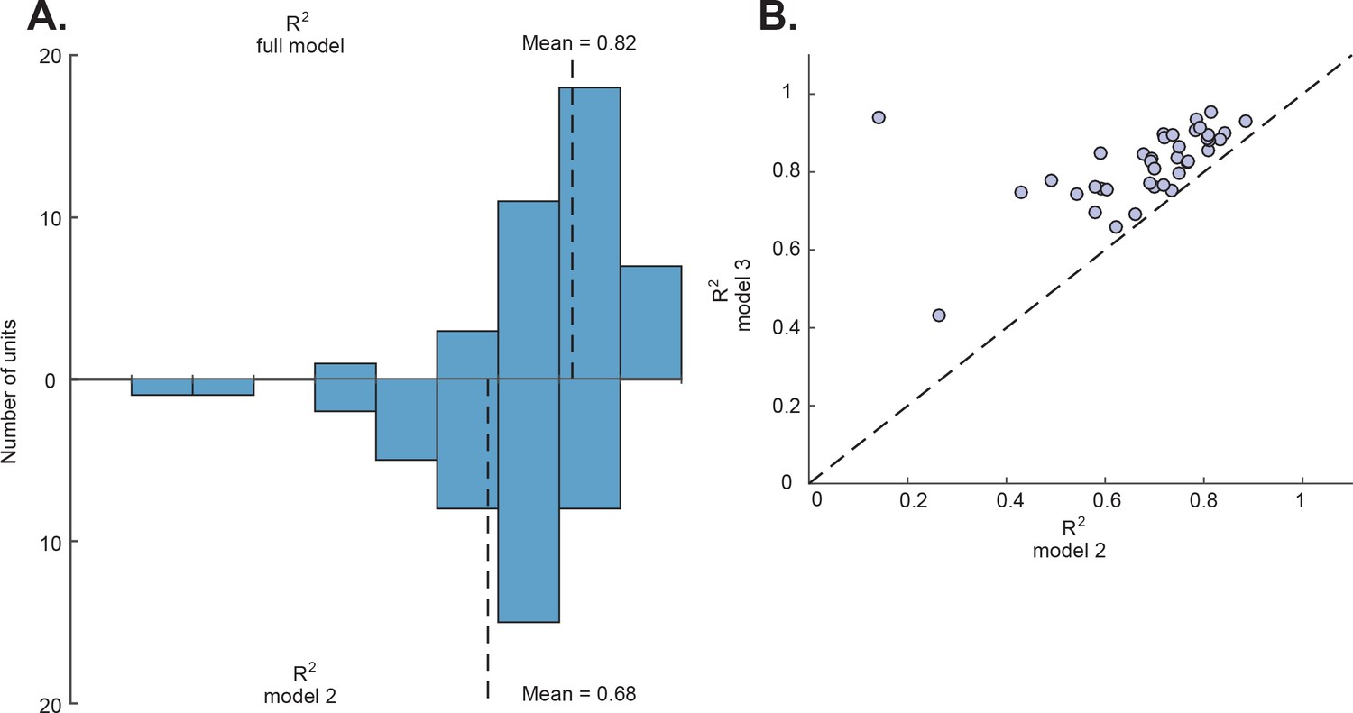
The comparison between the full model and model 2.
(A) The distributions of r2 of the full model (top) and model 2 (bottom). (B) The comparison of the r2 of the full model and model 2 for each neuron.
Tables
Table 1
Numbers of OFC neurons recorded and classified in this study.
For neurons with significant attentional modulation, we defined the consistency of the modulation as whether their responses to the double-cue conditions with visual perturbation became more or less similar to their responses to the single-cue condition when the perturbed cue was presented alone.
| Value-selective neurons | Positively tuned neurons | Negatively tuned neurons | Visually responsive neurons | Total# neurons recorded | ||
|---|---|---|---|---|---|---|
| No attentional modulation | 67 | 44 | 23 | 232 | 846 | |
| With attentional modulation | Consistent | 40 | 28 | 12 | ||
| Inconsistent | 3 | 1 | 2 | |||
| Total | 43 | 29 | 14 | |||
| Total | 110 | 73 | 37 | |||
Additional files
-
Supplementary files 1
includes Supplementary Tables 1–3.
- https://doi.org/10.7554/eLife.31507.024
-
Transparent reporting form
- https://doi.org/10.7554/eLife.31507.025
Download links
A two-part list of links to download the article, or parts of the article, in various formats.
Downloads (link to download the article as PDF)
Open citations (links to open the citations from this article in various online reference manager services)
Cite this article (links to download the citations from this article in formats compatible with various reference manager tools)
Covert shift of attention modulates the value encoding in the orbitofrontal cortex
eLife 7:e31507.
https://doi.org/10.7554/eLife.31507


