Sensory cortex is optimized for prediction of future input
- University of Oxford, United Kingdom
- City University of Hong Kong, Hong Kong
Figures
Figure 1

Temporal prediction model implemented using a feedforward artificial neural network, with the same architecture in both visual and auditory domains.
(a), Network trained on cochleagram clips (spectral content over time) of natural sounds, aims to predict immediate future time steps of each clip from recent past time steps. (b), Network trained on movie clips of natural scenes, aims to predict immediate future frame of each clip from recent past frames. , input – the past; , input weights; , hidden unit output; , output weights; , output – the predicted future; , target output – the true future. Hidden unit’s RF is the between the input and that unit .
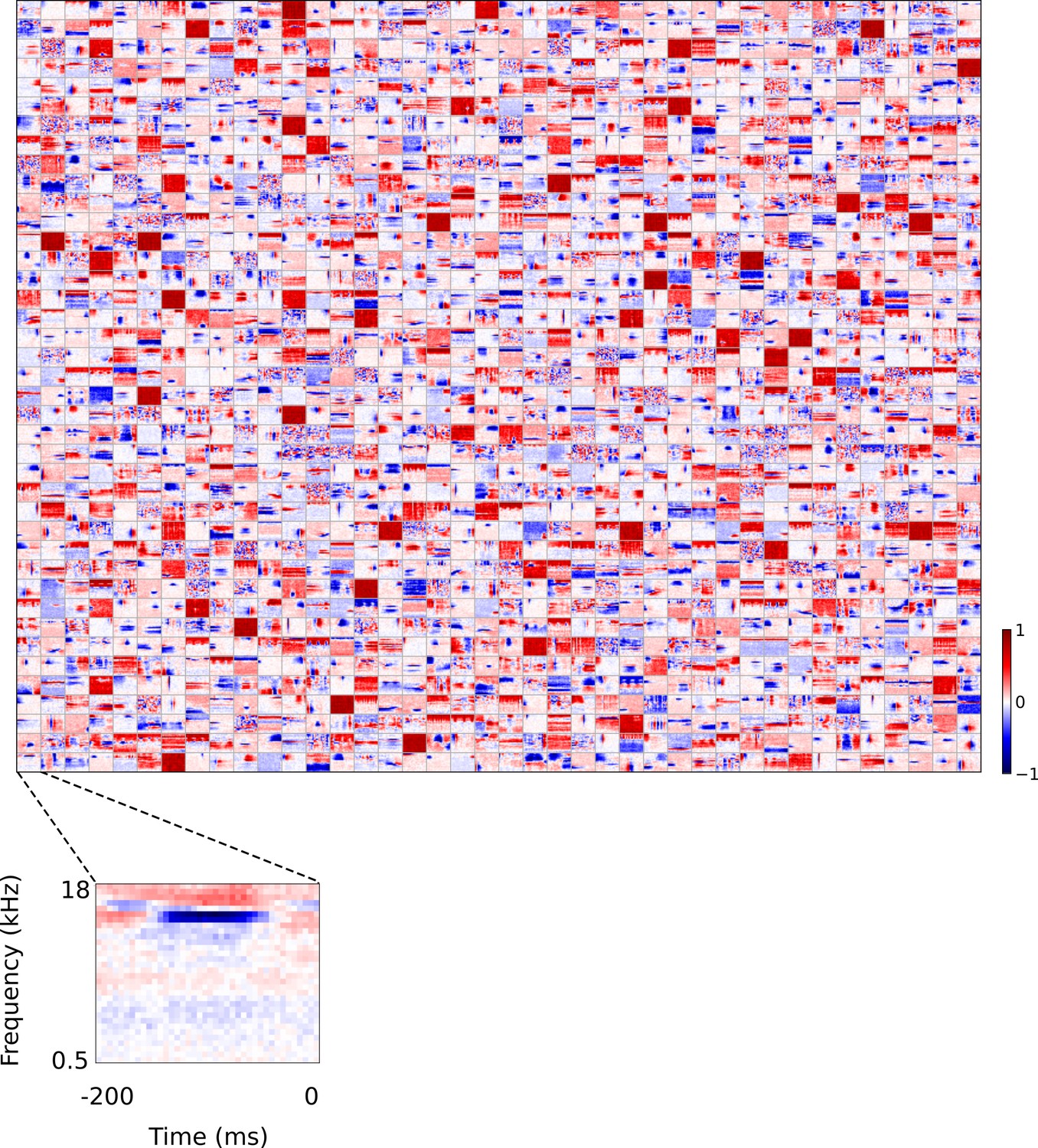
Figure 2
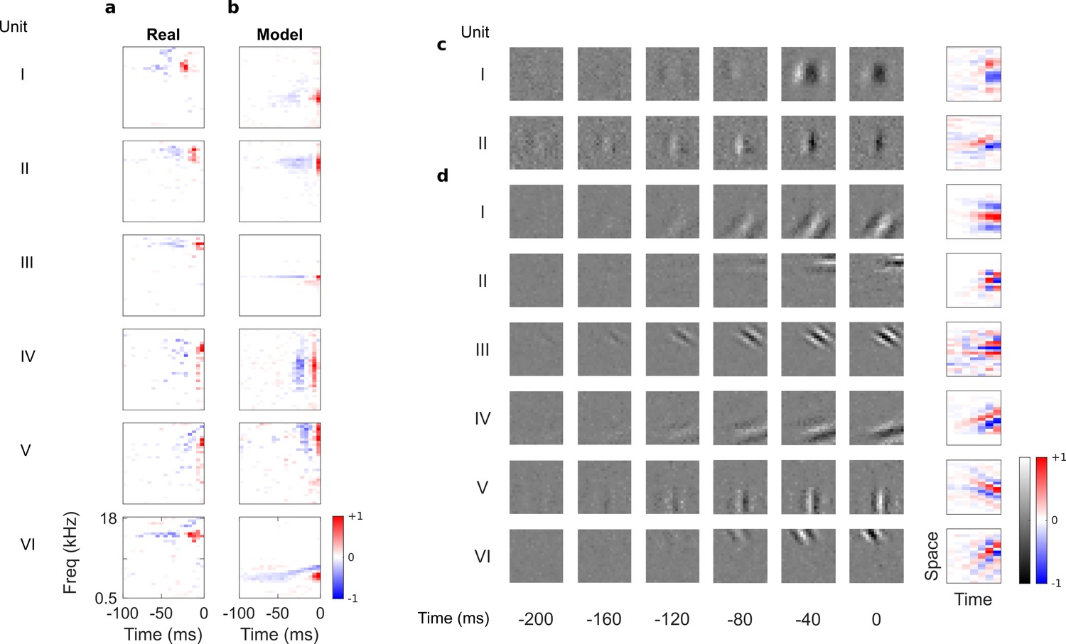
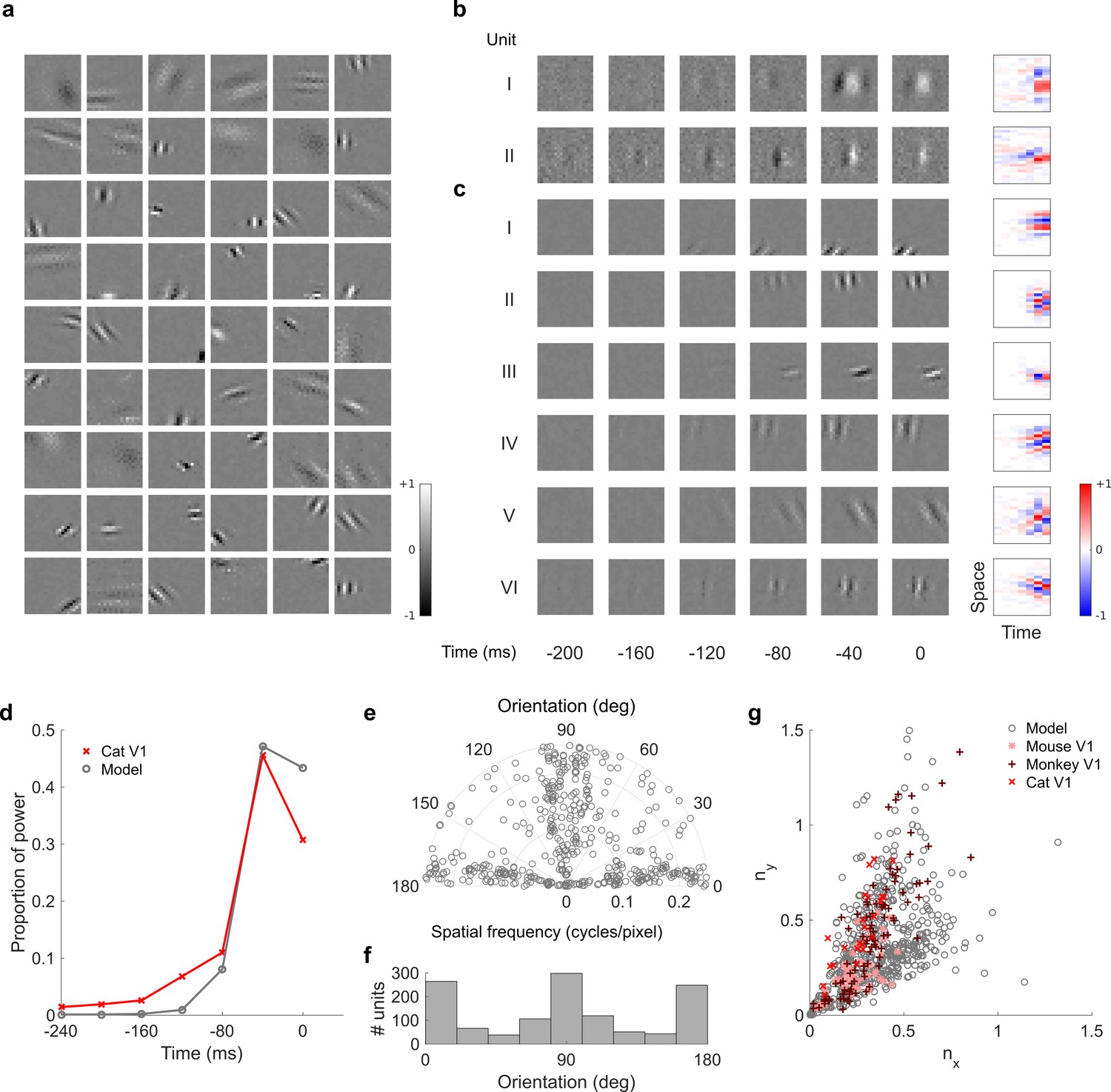
Auditory spectrotemporal and visual spatiotemporal RFs of real neurons and temporal prediction model units.
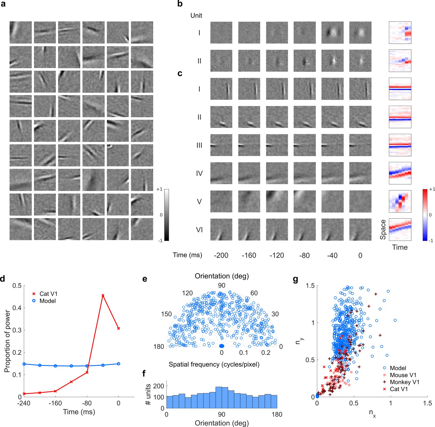
(a), Example spectrotemporal RFs of real A1 neurons (Willmore et al., 2016). Red – excitation, blue – inhibition. Most recent two time steps (10 ms) were removed to account for conduction delay. (b), Example spectrotemporal RFs of model units when model is trained to predict the future of natural sound inputs. Note that the overall sign of a receptive field learned by the model is arbitrary. Hence, in all figures and analyses we multiplied each model receptive field by −1 where appropriate to obtain receptive fields which all have positive leading excitation (see Materials and methods). (c), Example spatiotemporal (I, space-time separable, and II, space-time inseparable) RFs of real V1 neurons (Ohzawa et al., 1996). Left, grayscale: 3D (space-space-time) spatiotemporal RFs showing the spatial RF at each of the most recent six time steps. Most recent time step (40 ms) was removed to account for conduction delay. White – excitation, black – inhibition. Right: corresponding 2D (space-time) spatiotemporal RFs obtained by summing along the unit’s axis of orientation for each time step. Red – excitation, blue – inhibition. (d), Example 3D and corresponding 2D spatiotemporal (I-III, space-time separable, and IV-VI, space-time inseparable) RFs of model units when model is trained to predict the future of natural visual inputs.
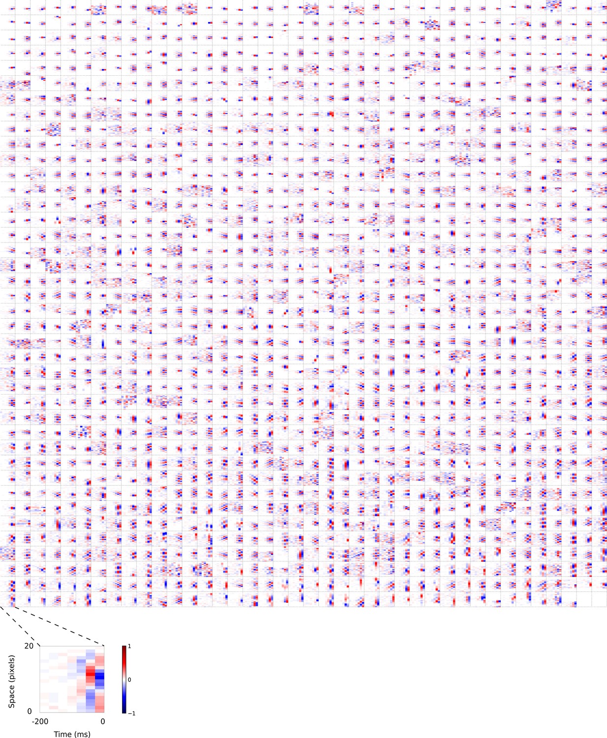
Figure 3
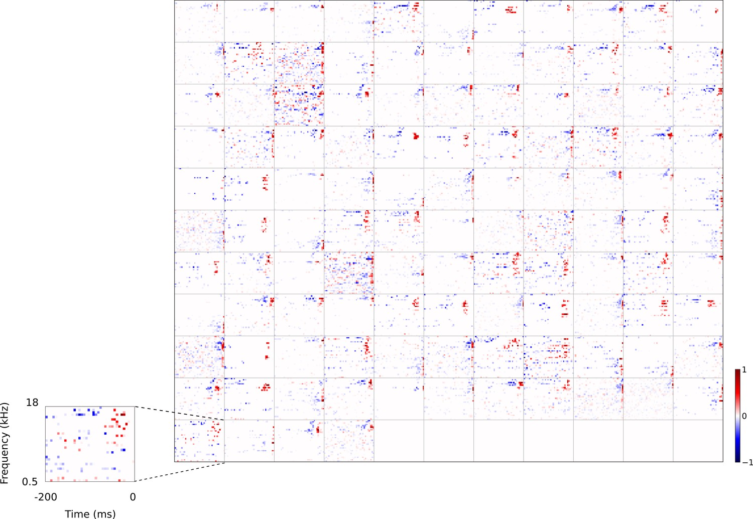
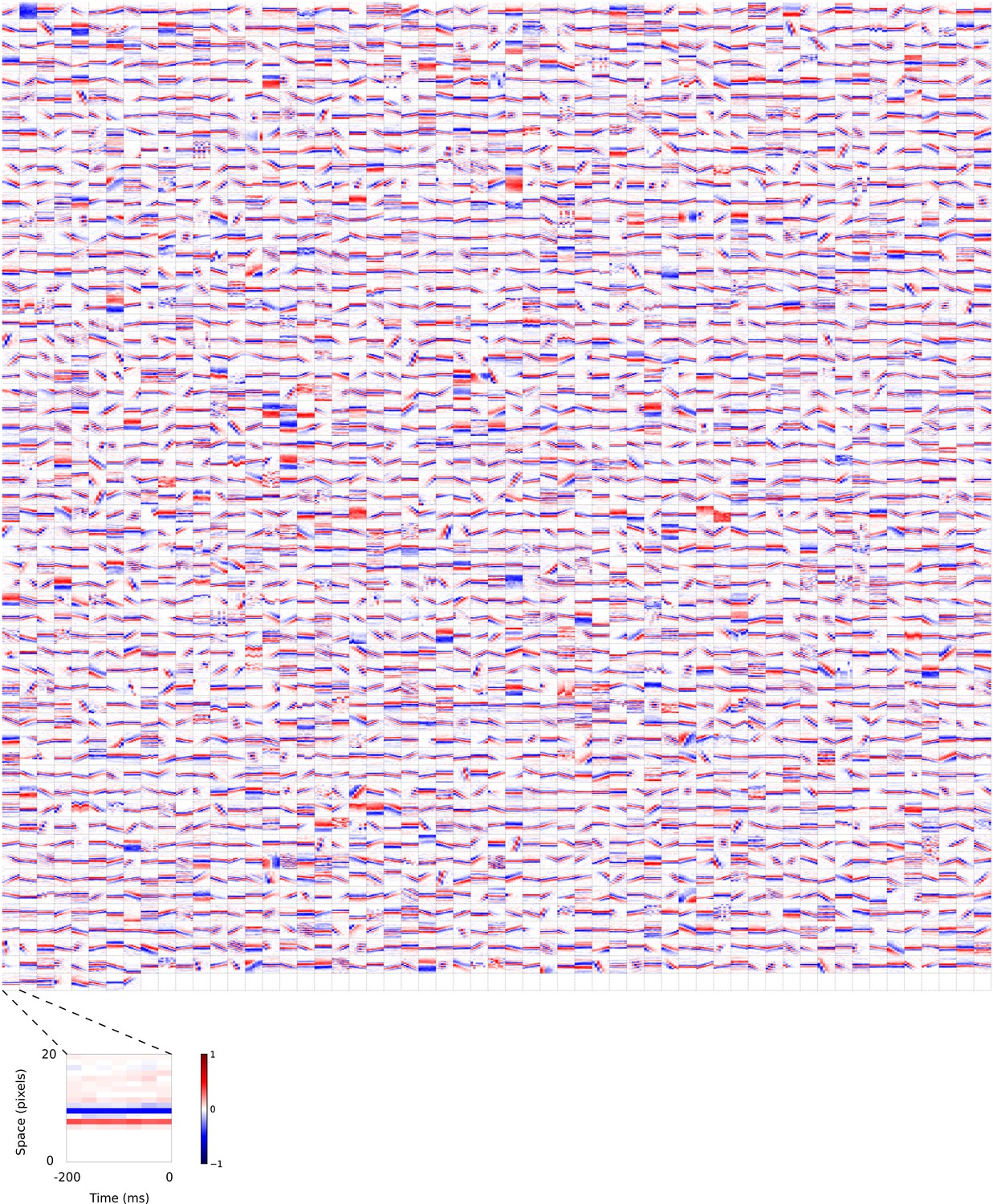
Full dataset of real auditory RFs.
114 neuronal RFs recorded from A1 and AAF of 5 ferrets. Red – excitation, blue - inhibition. Inset shows axes.
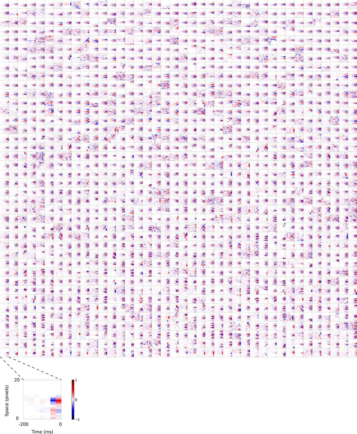
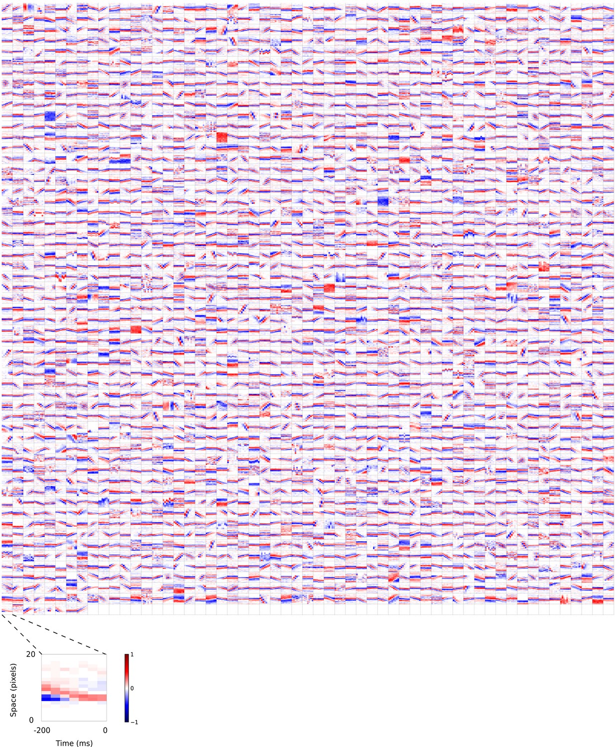
Figure 4 with 7 supplements
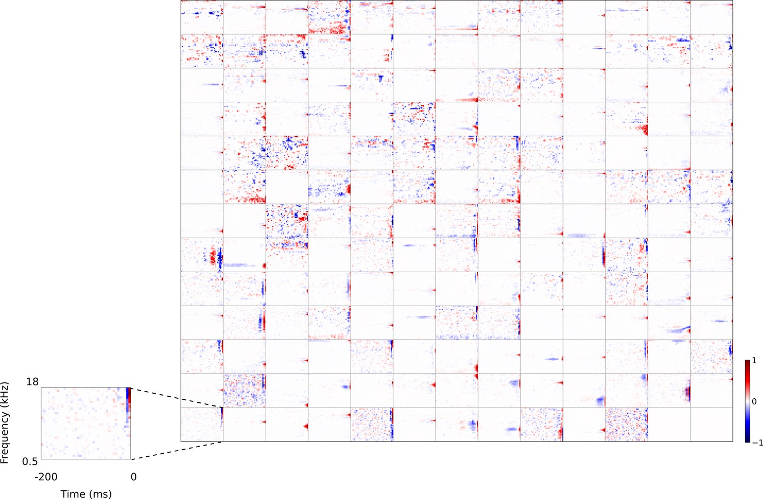
Full set of auditory RFs of the temporal prediction model units.
Units were obtained by training the model with 1600 hidden units on auditory inputs. The hidden unit number and L1 weight regularization strength (10−3.5) was chosen because it results in the lowest MSE on the prediction task, as measured using a cross validation set. Many hidden units’ weight matrices decayed to near zero during training (due to the L1 regularization), leaving 167 active units. Inactive units were excluded from analysis and are not shown. Example units in Figure 2 come from this set. Red – excitation, blue - inhibition. Inset shows axes. Figure 4—figure supplement 1 shows the same RFs on a finer timescale. The full sets of visual spatial and corresponding spatiotemporal RFs for the temporal prediction model when it is trained on visual inputs are shown in Figure 4—figure supplements 2–3. Figure 4—figure supplement 4 shows the auditory RFs of the temporal prediction model when a linear activation function instead of a sigmoid nonlinearity was used. Figure 4—figure supplement 5–7 show the auditory spectrotemporal and visual spatial and 2D spatiotemporal RFs of the temporal prediction model when it was trained on inputs without added noise.
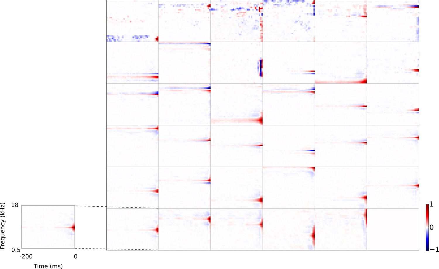
Figure 4—figure supplement 1
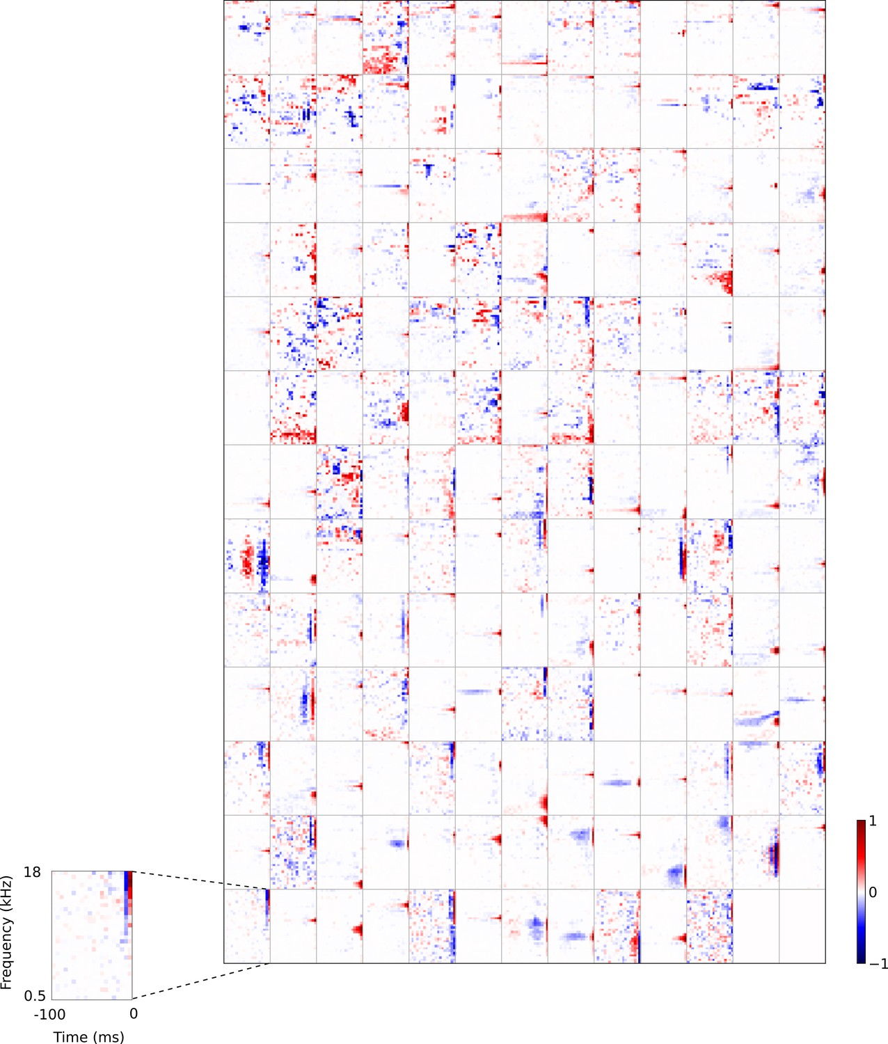
Full set of auditory RFs of the temporal prediction model units shown on a finer timescale.
All details are as in Figure 3, but the only the most recent 100 ms of the response profile is shown in order to illustrate details of the RFs. Inset shows axes.
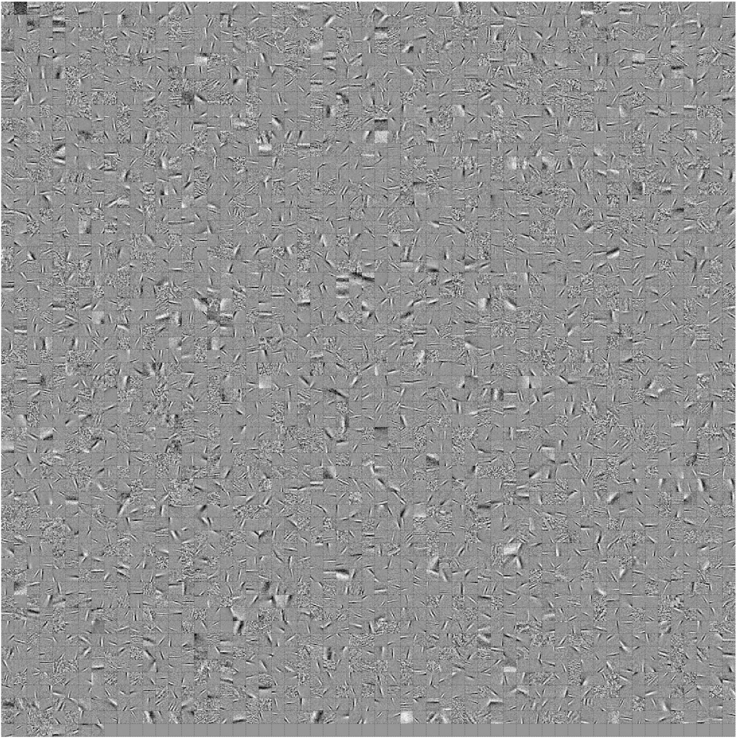
Figure 4—figure supplement 2
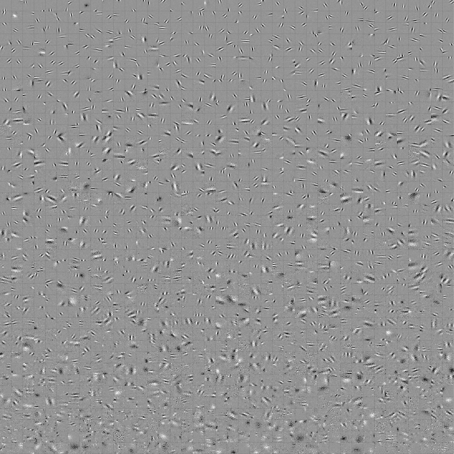
Full set of visual spatial RFs of the temporal prediction model units.
Units in Figures 2,7 come from this set. Each square represents the spatial RF of a single unit, shown at its best time step. The best time step was determined by selecting the time step for which the power (sum of squares) of the RF was greatest. White – excitation, black - inhibition.
Figure 4—figure supplement 3
Visual 2D (space-time) spatiotemporal RFs of temporal prediction model units.
Units in Figures 2,7 come from this set. M . Each square represents the 2D spatiotemporal RF of a single unit corresponding to the unit in the same position in Figure 4—figure supplement 2, obtained by summing across space along the axis of the orientation for that unit. Red – excitation, blue - inhibition. Inset shows axes.
Figure 4—figure supplement 4
Full set of auditory RFs of the temporal prediction model units using a linear activation function.
Units were obtained by training the model with 1600 hidden units on auditory inputs. The hidden unit number and L1 weight regularization strength (10−3.25) was chosen because they result in the lowest MSE on the prediction task, as measured using a cross validation set. Almost all hidden units’ weight matrices decayed to near zero during training (due to the L1 regularization), leaving 35 active units. Inactive units were excluded from analysis and are not shown. Red – excitation, blue - inhibition. Inset shows axes.
Figure 4—figure supplement 5
Full set of auditory RFs of the temporal prediction model units trained on auditory inputs without added noise.
Units were obtained by training the model with 1600 hidden units on auditory inputs. The hidden unit number and L1 weight regularization strength (10−4) was chosen because it results in the lowest MSE on the prediction task, as measured using a cross validation set. Many hidden units’ weight matrices decayed to near zero during training (due to the L1 regularization), leaving 465 active units. Inactive units were excluded from analysis and are not shown. Red – excitation, blue - inhibition. Inset shows axes.
Figure 4—figure supplement 6

Full set of visual spatial RFs of temporal prediction model units trained on visual inputs without added noise.
Model units were obtained by training the model with 1600 hidden units on visual inputs. The hidden unit number and L1 weight regularization strength (10−6.25) was chosen because it results in the lowest MSE on the prediction task, as measured using a cross validation set. Some hidden units’ weight matrices decayed to near zero during training (due to the L1 regularization), leaving 1585 active units, which were included in analysis. Inactive units were excluded from analysis. Each square represents the spatial RF of a single unit, shown at its best time step. The best time step was determined by selecting the time step for which the power (sum of squares) of the RF was greatest. White – excitation, black - inhibition.
Figure 4—figure supplement 7
2D (space-time) visual spatiotemporal RFs of temporal prediction model units trained on visual inputs without added noise.
Obtained from the same units shown in Figure 4—figure supplement 6 using methods outlined in Figure 2c. Red – excitation, blue - inhibition. Inset shows axes.
Figure 5 with 5 supplements
Full set of auditory ‘RFs’ (basis functions) of sparse coding model used as a control.
Units were obtained by training the sparse coding model with 1600 units on the identical auditory inputs used to train the network shown in Figure 4. L1 regularization of strength 100.5 was applied to the units’ activities. This network configuration was selected as it produced unit RFs that most closely resembled those recorded in A1, as determined using the KS measure of similarity Figure 8—figure supplement 1 . Although the basis functions of the sparse coding model are not receptive fields, but projective fields, they tend to be similar in structure (Olshausen and Field, 1996, Olshausen and Field, 1997). In this manuscript, to have a common term between models and the data, we refer to sparse coding basis functions as RFs. Red – excitation, blue - inhibition. Inset shows axes. The full sets of visual spatial and corresponding spatiotemporal RFs for the sparse coding model when it is trained on visual inputs are shown in Figure 5—figure supplements 1–2. Figure 5—figure supplements 3–5 show the auditory spectrotemporal and visual spatial and 2D spatiotemporal RFs of the sparse coding model when it was trained on inputs without added noise.
Figure 5—figure supplement 1

Full set of visual spatial RFs of sparse coding model units.
Model units were obtained by training the sparse coding model with 3200 units on identical visual inputs used to train the temporal prediction model Figure 4—figure supplement 2. The model configuration (3200 units, L1 sparsity strength of 100.5 on the unit activities) was chosen because it resulted in the RFs that look most like the RFs of V1 simple cells as determined by visual inspection. Each square represents the spatial RF of a single unit, shown at its best time step. The best time step was determined by selecting the time step for which the power (sum of squares) of the RF was greatest. White – excitation, black - inhibition.
Figure 5—figure supplement 2
2D (space-time) visual spatiotemporal RFs of sparse coding model units.
Obtained from the same units shown in Figure 5—figure supplement 1 using methods outlined in Figure 2c. Red – excitation, blue - inhibition. Inset shows axes.
Figure 5—figure supplement 3

Full set of auditory RFs of sparse coding model trained on auditory inputs without added noise.
Units were obtained by training the sparse coding model with 1600 units on the identical auditory inputs used to train the network shown in Figure 4—figure supplement 5. L1 regularization of strength 100.5 was applied to the units’ activities. This network configuration was selected as it produced unit RFs that most closely resembled those recorded in A1, as determined by visual inspection. Red – excitation, blue - inhibition. Inset shows axes.
Figure 5—figure supplement 4
Full set of visual spatial RFs of sparse coding model units trained on visual inputs without added noise.
Model units were obtained by training the sparse coding model with 3200 units on identical visual inputs used to train the temporal prediction model Figure 4—figure supplement 6. The model configuration (3200 units, L1 sparsity strength of 100.5 on the unit activities) was chosen because it resulted in the RFs that look most like the RFs of V1 simple cells as determined by visual inspection. Each square represents the spatial RF of a single unit, shown at its best time step. The best time step was determined by selecting the time step for which the power (sum of squares) of the RF was greatest. White – excitation, black - inhibition.
Figure 5—figure supplement 5
2D (space-time) visual spatiotemporal RFs of sparse coding model units trained on visual inputs without added noise.
Obtained from the same units shown in Figure 5—figure supplement 4 using methods outlined in Figure 2c. Red – excitation, blue - inhibition. Inset shows axes.
Figure 6 with 1 supplement

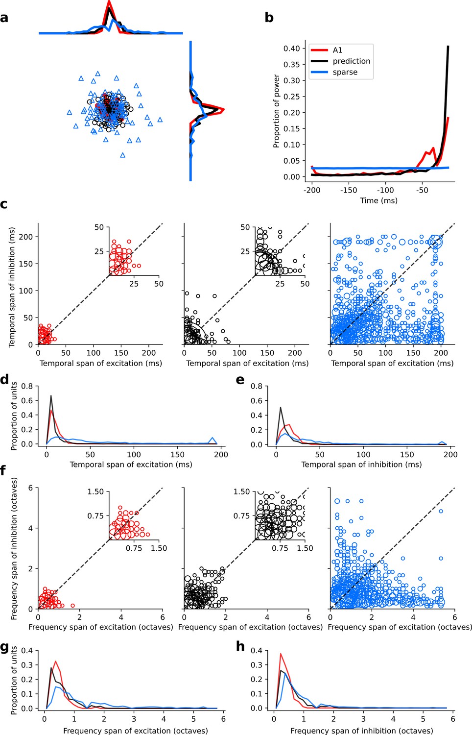
Population measures for real A1, temporal prediction model and sparse coding model auditory spectrotemporal RFs.
The population measures are taken from the RFs shown in Figures 3–5. (a), Each point represents a single RF (with 32 frequency and 38 time steps) which has been embedded in a 2-dimensional space using Multi-Dimensional Scaling (MDS). Red circles - real A1 neurons, black circles – temporal prediction model units, blue triangles – sparse coding model units. Colour scheme applies to all subsequent panels. (b), Proportion of power contained in each time step of the RF, taken as an average across the population of units. (c), Temporal span of excitatory subfields versus that of inhibitory subfields, for real neurons and temporal prediction and sparse coding model units. The area of each circle is proportional to the number of occurrences at that point. The inset plots, which zoom in on the distribution use a smaller constant of proportionality for the circles to make the distributions clearer. (d), Distribution of temporal spans of excitatory subfields, taken by summing along the x-axis in (c). (e), Distribution of temporal spans of inhibitory subfields, taken by summing along the y-axis in (c). (f), Frequency span of excitatory subfields versus that of inhibitory subfields, for real neurons and temporal prediction and sparse coding model units. (g), Distribution of frequency spans of excitatory subfields, taken by summing along the x-axis in (f). (h), Distribution of frequency spans of inhibitory subfields, taken by summing along the y-axis in (f). Figure 6—figure supplement 1 shows the same analysis for the temporal prediction model and sparse coding model trained on auditory inputs without added noise.
Figure 6—figure supplement 1
Population measures for real A1, temporal prediction model and sparse coding model auditory spectrotemporal RFs when models are trained on auditory inputs without added noise.
Real units are the same as those shown in Figure 3. Temporal prediction model units are the same as those shown in Figure 4—figure supplement 5. Sparse coding model units are the same as those shown in Figure 5—figure supplement 3. (a), Each point represents a single RF (with 32 frequency and 38 time steps) which has been embedded in a two dimensional space using Multi-Dimensional Scaling (MDS). Red circles - real A1 neurons, black circles – temporal prediction model units, blue triangles – sparse coding model units. Colour scheme applies to all subsequent panels in Figure. (b), Proportion of power contained in each time step of the RF, taken as an average across the population of units. (c), Temporal span of excitatory subfields versus that of inhibitory subfields, for real neurons and temporal prediction and sparse coding model units. The area of each circle is proportional to the number of occurrences at that point. The inset plots, which zoom in on the distribution use a smaller constant of proportionality for the circles to make the distributions clearer. (d), Distribution of temporal spans of excitatory subfields, taken by summing along the x-axis in (c). (e), Distribution of temporal spans of inhibitory subfields, taken by summing along the y-axis in (c). (f), Frequency span of excitatory subfields versus that of inhibitory subfields, for real neurons and temporal prediction and sparse coding model units. (g) Distribution of frequency spans of excitatory subfields, taken by summing along the x-axis in (f). (h), Distribution of frequency spans of inhibitory subfields, taken by summing along the y-axis in (f). The addition of noise leads to subtle changes in the RFs. Without noise, the inhibition in the temporal prediction model tends to be slightly less extended and the RFs a little less smooth (see Figure 4, Figure 4—figure supplement 5 for qualitative comparison).
Figure 7 with 3 supplements
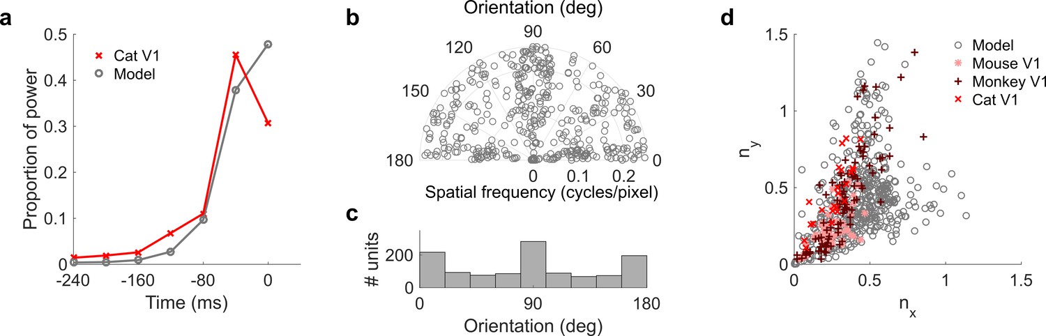
Population measures for real V1 and temporal prediction model visual spatial and spatiotemporal RFs.
Model units were obtained by training the model with 1600 hidden units on visual inputs. The hidden unit number and L1 weight regularization strength (10−6.25) was chosen because it results in the lowest MSE on the prediction task, as measured using a cross validation set. Example units in Figure 2 come from this set. (a), Proportion of power (sum of squared weights over space and averaged across units) in each time step, for real (Ohzawa et al., 1996) and model populations. (b), Joint distribution of spatial frequency and orientation tuning for population of model unit RFs at their time step with greatest power. (c), Distribution of orientation tuning for population of model unit RFs at their time step with greatest power. (d), Distribution of RF shapes for real neurons (cat, Jones and Palmer, 1987, mouse, Niell and Stryker, 2008 and monkey, Ringach, 2002) and model units. nx and ny measure RF span parallel and orthogonal to orientation tuning, as a proportion of spatial oscillation period (Ringach, 2002). For (b–d), only units that could be well approximated by Gabor functions (n = 1205 units; see Materials and methods) were included in the analysis. Of these, only model units that were space-time separable (n = 473) are shown in (d) to be comparable with the neuronal data (Ringach, 2002). A further 4 units with 1.5 < ny < 3.1 are not shown in (d). Figure 7—figure supplements 1–3 show example visual RFs and the same population measures for the sparse coding model trained on visual inputs with added noise and for the temporal prediction and sparse coding models trained on visual inputs without added noise.
Figure 7—figure supplement 1

Visual RFs and population measures for real V1 neurons and sparse coding model units.
Model units are the same as those used in Figure 5—figure supplement 1; Figure 5—figure supplement 2. (a), Example spatial RFs of randomly selected units at their best time step. (b–c), Example 3D and corresponding 2D spatiotemporal RFs at most recent six time steps of (b) (I, space-time separable, and II, space-time inseparable) real (Rao and Ballard, 1999) V1 neurons and (c) (I-III, space-time separable, and IV-VI, space-time inseparable) sparse coding model units. (d), Proportion of power (sum of squared weights over space and averaged across units) in each time step, for real and model populations. (e), Joint distribution of spatial frequency and orientation tuning for population of model units. (f), Distribution of orientation tuning for population of model units. (f), Distribution of RF shapes for real neurons (cat, Jones and Palmer, 1987, mouse, Niell and Stryker, 2008, and monkey, Ringach, 2002) and model units. For (e–g), only units that could be well approximated by Gabor functions (n = 2402 units; see Materials and methods) were included in the analysis. Of these, only model units that were space-time separable (n = 881) are shown in (f) to be comparable with the neuronal data (Ringach, 2002).
Figure 7—figure supplement 2
Visual RFs and population measures for real V1 neurons and temporal prediction model units trained on visual inputs without added noise.
Model units are drawn from Figure 4—figure supplement 6; Figure 4—figure supplement 7 (a), Example spatial RFs of randomly selected units at their best time step. (b–c), Example 3D and corresponding 2D spatiotemporal RFs at most recent six time steps of (I, space-time separable, and II, space-time inseparable) real (Rao and Ballard, 1999) V1 neurons and (c) (I-III, space-time separable, and IV-VI, space-time inseparable) sparse coding model units. (d), Proportion of power (sum of squared weights over space and averaged across units) in each time step, for real and model populations. (e), Joint distribution of spatial frequency and orientation tuning for population of model units. (f), Distribution of orientation tuning for population of model units. (g), Distribution of RF shapes for real neurons (cat, Jones and Palmer, 1987, mouse, Niell and Stryker, 2008 and monkey, Ringach, 2002) and model units. For (e–g), only units that could be well approximated by Gabor functions (n = 1246 units; see Materials and methods) were included in the analysis. Of these, only model units that were space-time separable (n = 569) are shown in (g) to be comparable with the neuronal data (Ringach, 2002). The addition of noise only leads to subtle changes in the RFs; most apparently, there are more units with RFs comprising multiple short subfields (forming an increased number of points towards the lower right quadrant of (g) than is seen in the case when noise is used.
Figure 7—figure supplement 3
Visual RFs and population measures for real V1 neurons and sparse coding model units trained on visual inputs without added noise.
Model units are drawn from Figure 5—figure supplement 4; Figure 5—figure supplement 5. (a), Example spatial RFs of randomly selected units at their best time step. (b–c), Example 3D and corresponding 2D spatiotemporal RFs at most recent six time steps of (b) (I, space-time separable, and II, space-time inseparable) real (Rao and Ballard, 1999) V1 neurons and (c) (I-III, space-time separable, and IV-VI, space-time inseparable) sparse coding model units. (d), Proportion of power (sum of squared weights over space and averaged across units) in each time step, for real and model populations. (e), Joint distribution of spatial frequency and orientation tuning for population of model units. (f), Distribution of orientation tuning for population of model units. (g), Distribution of RF shapes for real neurons (cat,Jones and Palmer, 1987, mouse, Niell and Stryker, 2008, and monkey, Ringach, 2002) and model units. For (e–g), only units that could be well approximated by Gabor functions (n = 2482 units; see Materials and methods) were included in the analysis. Of these, only model units that were space-time separable (n = 860) are shown in (f) to be comparable with the neuronal data (Ringach, 2002).
Figure 8 with 3 supplements
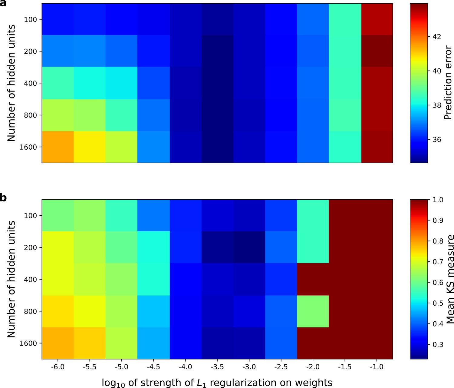
Correspondence between the temporal prediction model’s ability to predict future auditory input and the similarity of its units’ responses to those of real A1 neurons.
Performance of model as a function of number of hidden units and L1 regularization strength on the weights as measured by (a), prediction error (mean squared error) on the validation set at the end of training and (b), similarity between model units and real A1 neurons. The similarity between the real and model units is measured by averaging the Kolmogorov-Smirnov distance between each of the real and model distributions for the span of temporal and frequency tuning of the excitatory and inhibitory RF subfields (e.g. the distributions in Figure 6d–e and Figure 6g–h). Figure 8—figure supplement 1 shows the same analysis, performed for the sparse coding model, which does not produce a similar correspondence.
Figure 8—figure supplement 1
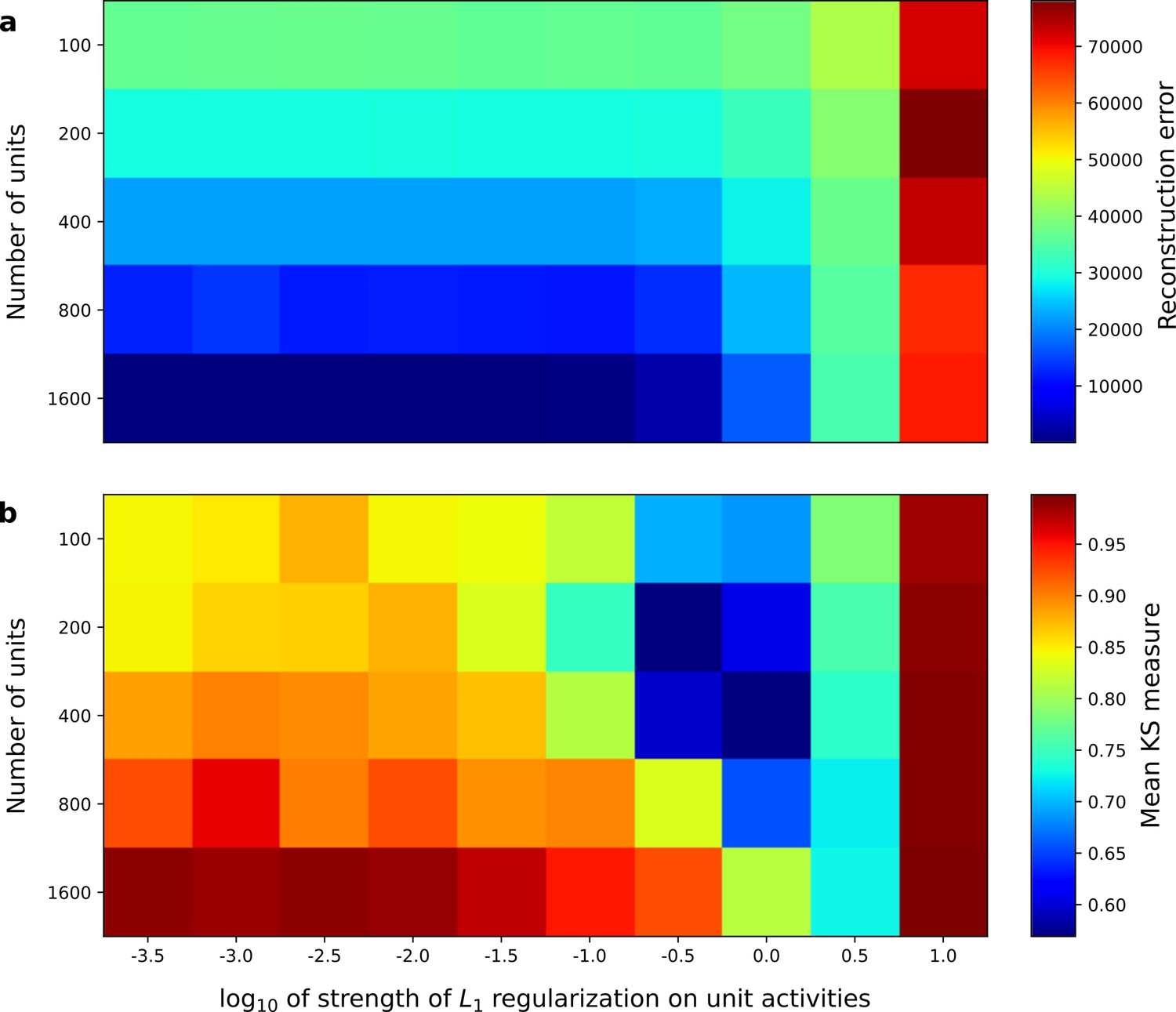
Correspondence between sparse coding model’s ability to reproduce its input and the similarity of its units’ responses to those of real A1 neurons.
Performance of model as a function of number of units and the L1 regularization strength on the activities as measured by (a), reconstruction error (mean squared error) on the validation set at the end of training and (b), similarity between model units and real A1 neurons. The similarity between the real and model units is measured by averaging the Kolmogorov-Smirnov distance between each of the real and model distributions for the span of temporal and frequency tuning of the excitatory and inhibitory RF subfields (e.g. the distributions in Figure 3d–e and Figure 3g–h).
Figure 8—figure supplement 2
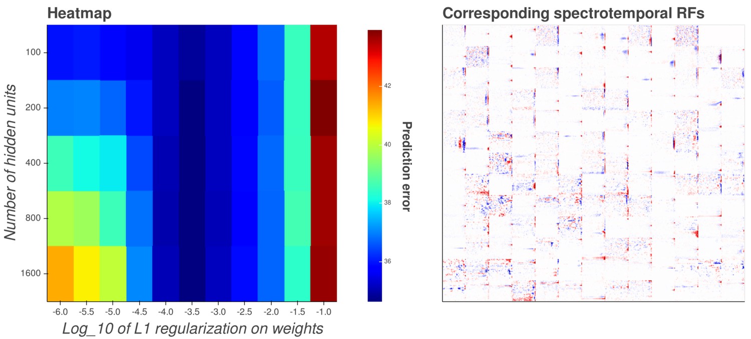
Interactive figure exploring the relationship between the strength of L1 regularization on the network weights and the structure of the RFs the network produces when the network is trained on auditory inputs.
The interactive version of this figure can be found at https://yossing.github.io/temporal_prediction_model/figures/interactive_supplementary_figures.html. The left hand panel shows the performance of the network with the hyperparameter settings specified on the x and y axes. The x axis signifies the strength of L1 regularization placed on the weights of the network during training. The y axis signifies the number of hidden units in the network. The colour represents the predictive capacity of the model as measured by the prediction error (mean squared error) on the validation set at the end of training.
How to interact with the figure: Hover over a point in the left hand panel to show the corresponding spectrotemporal receptive fields of the network in the right hand panel. Using the settings near the right hand panel, zoom, pan and reset the image to explore the shapes of the spectrotemporal receptive fields. Many hidden units’ weight matrices decayed to near zero during training. Inactive units were excluded from analysis and are not shown.
Figure 8—figure supplement 3
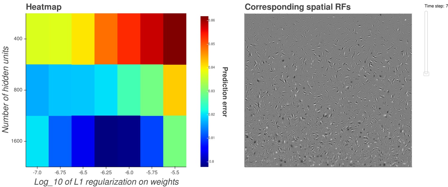
Interactive figure exploring the relationship between the strength of L1 regularization on the network weights and the structure of the RFs the network produces when the network is trained on visual inputs.
The interactive version of this figure can be found at: https://yossing.github.io/temporal_prediction_model/figures/interactive_supplementary_figures.html. The left hand panel shows the performance of the network with the hyperparameter settings specified on the x and y axes. The x axis signifies the strength of L1 regularization placed on the weights of the network during training. The y axis signifies the number of hidden units in the network. The colour represents the predictive capacity of the model as measured by the prediction error (mean squared error) on the validation set at the end of training.
How to interact with the figure: Hover over a point in the left panel to show the corresponding spatial receptive fields of the network in the right panel. Using the settings on the right of the right hand panel, zoom, pan and reset the image to explore the shapes of the spatial receptive fields. Change the slider labelled 'time step' to change the time-step of the spatial receptive fields shown in the right hand panel. Some hidden units’ weight matrices decayed to near zero during training. Inactive units were excluded from analysis and are not shown.
Additional files
-
Transparent reporting form
- https://doi.org/10.7554/eLife.31557.030
Download links
A two-part list of links to download the article, or parts of the article, in various formats.
Downloads (link to download the article as PDF)
Open citations (links to open the citations from this article in various online reference manager services)
Cite this article (links to download the citations from this article in formats compatible with various reference manager tools)
Sensory cortex is optimized for prediction of future input
eLife 7:e31557.
https://doi.org/10.7554/eLife.31557


