Figures and data in Cerebellar learning using perturbations

Figures
Tables
Additional files

13 figures, 2 tables and 1 additional file

Figures

Figure 1

Download asset Open asset

The cerebellar circuitry and properties of Purkinje cells.

(A) Simplified circuit diagram. MF, mossy fibres; CN, (deep) cerebellar nuclei; GC, granule cells; Cb Ctx, cerebellar cortex; PF, parallel fibres; PC, Purkinje cells; PN, projection neurones; NO, nucleo-olivary neurones; IO, inferior olive; CF, Climbing fibres. (B) Modular diagram. The $\pm$ signs next to the synapses indicate whether they are excitatory or inhibitory. The granule cell and indirect inhibitory inputs they recruit have been subsumed into a bidirectional mossy fibre–Purkinje cell input, M. Potentially plastic inputs of interest here are denoted with an asterisk. $i$ , input; $o$ , output; $ℰ (o)$ , error (which is a function of the output). (C) Typical Purkinje cell electrical activity from an intracellular patch-clamp recording. Purkinje cells fire two types of action potential: simple spikes and, in response to climbing fibre input, complex spikes. (D) According to the consensus plasticity rule, a complex spike will depress parallel fibre synapses active about 100 ms earlier. The diagram depicts idealised excitatory postsynaptic currents (EPSCs) before and after typical induction protocols inducing long-term potentiation (LTP) or depression (LTD). Grey, control EPSC; blue, green, post-induction EPSCs.

https://doi.org/10.7554/eLife.31599.002

Figure 2

Download asset Open asset

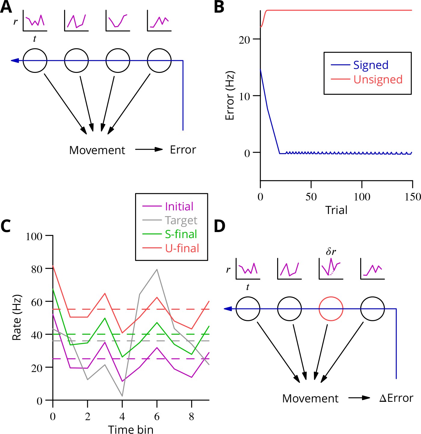
Analysis of cerebellar learning.

(A) The model of cerebellar learning we address is to adjust the temporal firing profiles (miniature graphs of rate as a function of time, $r (t)$ , *magenta*) of multiple cerebellar output neurones (nuclear projection neurones) (*black circles*) to optimise a movement, exploiting the evaluated movement error, which is fed back to the cerebellar circuit (Purkinje cells) (*blue arrow*). (B) The Marr-Albus-Ito theory was simulated in a network simulation embodying different error definitions (Results, Materials and methods). The Marr-Albus-Ito algorithm is able to minimise the average signed error (*blue*, *Signed*) of a group of projection neurones, but not the unsigned error (*red*, *Unsigned*). (C) However, as expected, optimising the signed error does not optimise individual cell firing profiles: comparison of the underlying firing profiles (initial, *magenta*; final, *green*) with their target (*grey*) for a specimen projection neurone illustrates that neither the temporal profile nor even the mean single-cell firing rate is optimised. If the unsigned error is used, there is no convergence and the firing rates simply saturate (*red*) and the error *increases*. (D) A different learning algorithm will be explored below: stochastic gradient descent, according to which temporally and spatially localised firing perturbations ( $δ r$ , *red*, of a Purkinje cell) are consolidated if the movement improves; this requires extraction of the *change* of error ( $Δ$ Error).

https://doi.org/10.7554/eLife.31599.003

Figure 3

Download asset Open asset

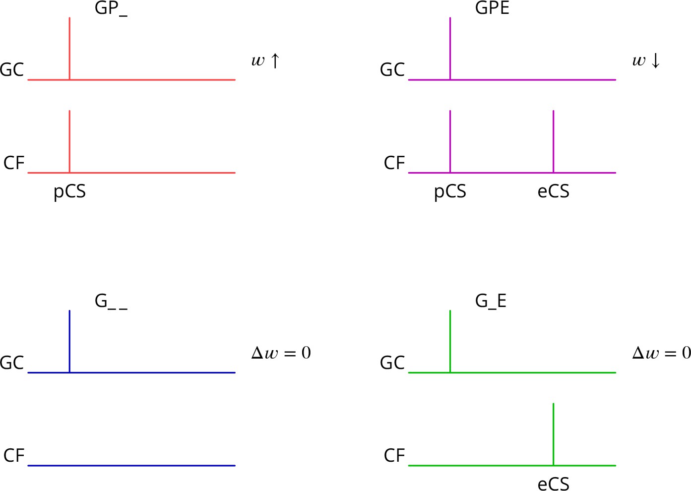
Predicted plasticity rules.

Synchronous activation of granule cell synapses and a perturbation complex spike (pCS) leads to LTP (GP_, increased synaptic weight $w$ ; top left, *red*), while the addition of a succeeding error complex spike (eCS) leads to LTD (GPE, top right, *magenta*). The bottom row illustrates the corresponding ‘control’ cases from which the perturbation complex spike is absent; no plasticity should result (G_ _ blue and G_E *green*).

https://doi.org/10.7554/eLife.31599.004

Figure 4

Download asset Open asset

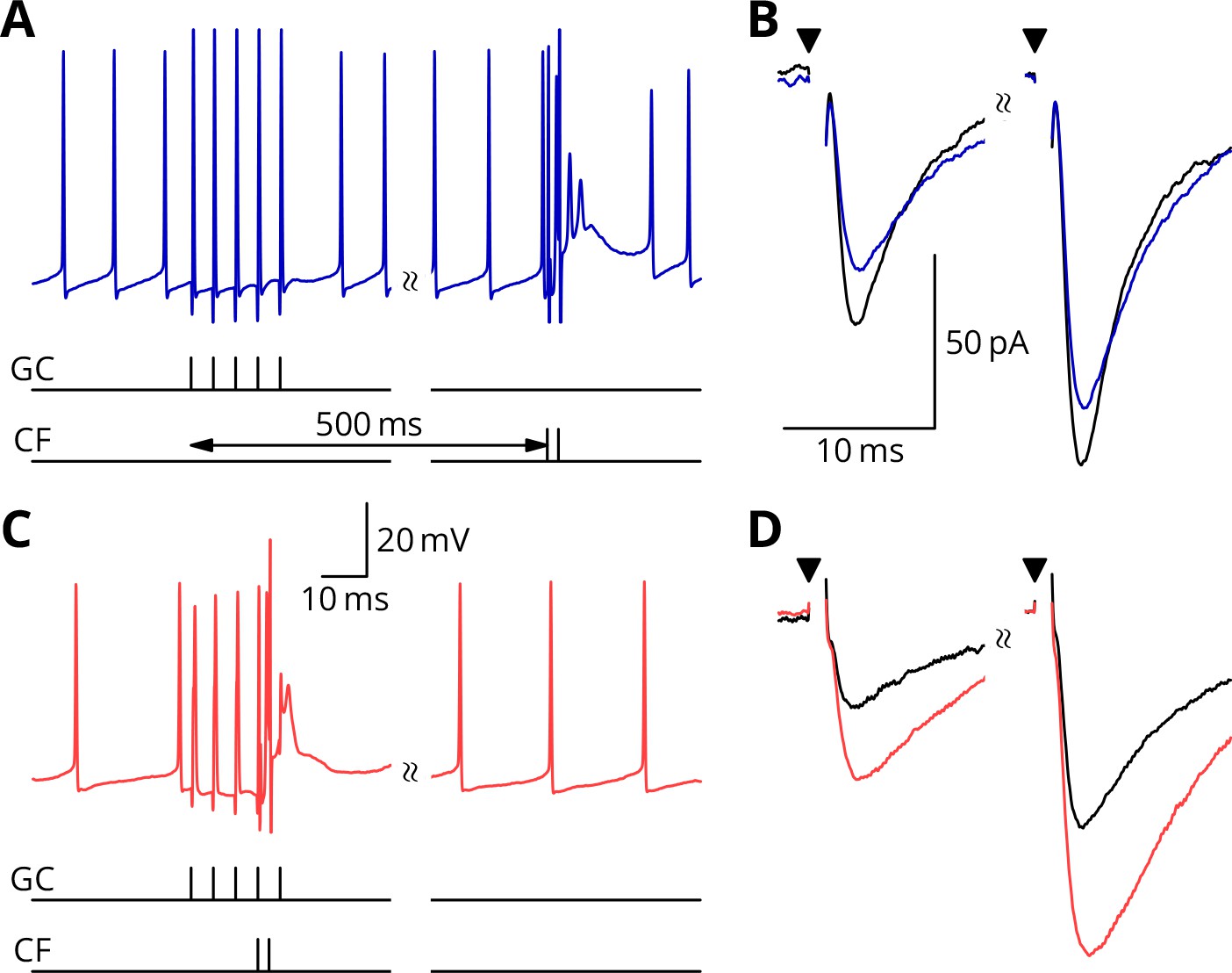
Simultaneous granule cell and climbing fibre activity induces LTP.

(A) Membrane potential (*blue*) of a Purkinje cell during an induction protocol (G_ _) where a burst of 5 granule cell stimuli at 200 Hz was followed after 0.5 s by a pair of climbing fibre stimuli at 400 Hz. (B) Average EPSCs recorded up to 10 min before (*black*) and 20–30 min after the end of the protocol of A (*blue*). Paired test stimuli (*triangles*) were separated by 50 ms and revealed the facilitation typical of the granule cell input to Purkinje cells. In this case, the induction protocol resulted in a small reduction (*blue* vs. *black*) of the amplitude of responses to both pulses. (C) Purkinje cell membrane potential (*red*) during a protocol (GP_) where the granule cells and climbing fibres were activated simultaneously, with timing otherwise identical to A. (D) EPSCs recorded before (*black*) and after (*red*) the protocol in C. A clear potentiation was observed in both of the paired-pulse responses.

https://doi.org/10.7554/eLife.31599.005

Figure 5

Download asset Open asset

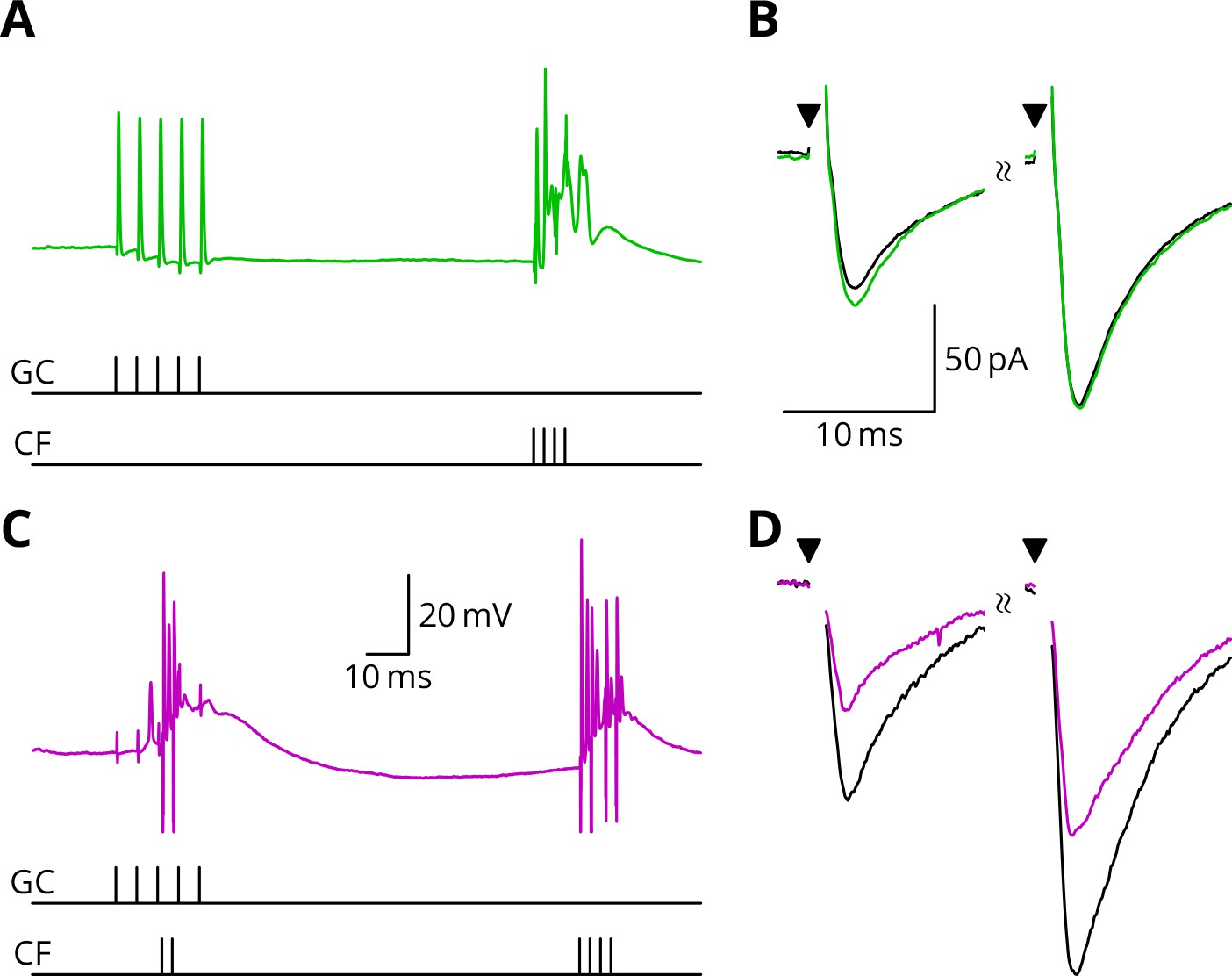
LTD requires simultaneous granule cell and climbing fibre activity closely followed by an additional complex spike.

(A) Membrane potential of a Purkinje cell (*green*) during a protocol where a burst of five granule cell stimuli at 200 Hz was followed after 100 ms by four climbing fibre stimuli at 400 Hz (G_E). (B) Average EPSCs recorded up to 10 min before (*black*) and 20–30 min after the end of the protocol of A (*green*). The interval between the paired test stimuli (*triangles*) was 50 ms. The induction protocol resulted in little change (*green* vs. *black*) of the amplitude of either pulse. (C) Purkinje cell membrane potential (*magenta*) during the same protocol as in A with the addition of a pair of climbing fibre stimuli simultaneous with the granule cell stimuli (GPE). (D) EPSCs recorded before (*black*) and after (*magenta*) the protocol in C. A clear depression was observed.

https://doi.org/10.7554/eLife.31599.006

Figure 6 with 1 supplement

Download asset Open asset

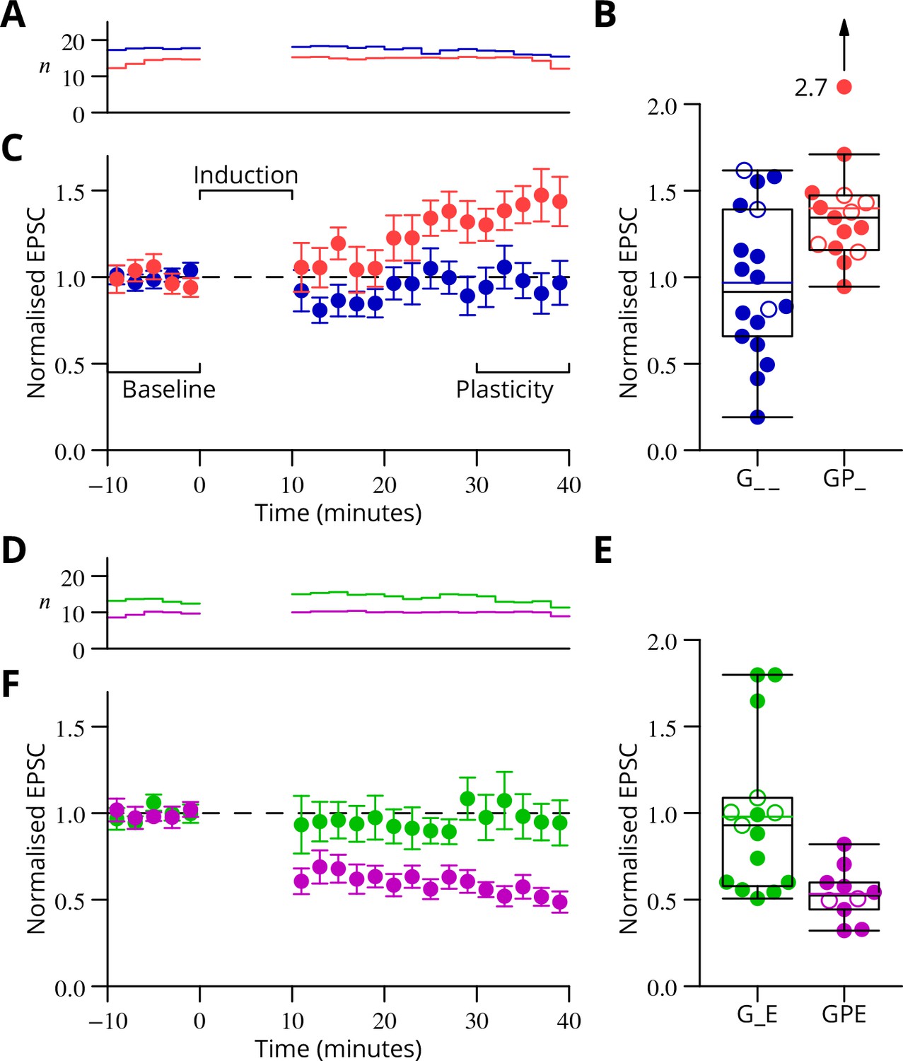
Time course and amplitude of plasticity.

(A) number, (B) box-and-whisker plots of individual plasticity ratios (*coloured lines* represent the means, *open symbols* represent cells with failures of climbing fibre stimulation; see Materials and methods) and (C) time course of the mean EPSC amplitude for GP_ (red) and G_ _ (blue) protocols of Figure 4, normalised to the pre-induction amplitude. Averages every 2 min, mean $\pm$ sem. Non-integer $n$ arise because the numbers of responses averaged were normalised by those expected in two minutes, but some responses were excluded (see Materials and methods) and some recordings did not extend to the extremities of the bins. Induction lasted for 10 min starting at time 0. (**D, E**) and (F) similar plots for the GPE (*magenta*) and G_E (*green*) protocols of Figure 5.

https://doi.org/10.7554/eLife.31599.007

Figure 6—figure supplement 1

Download asset Open asset

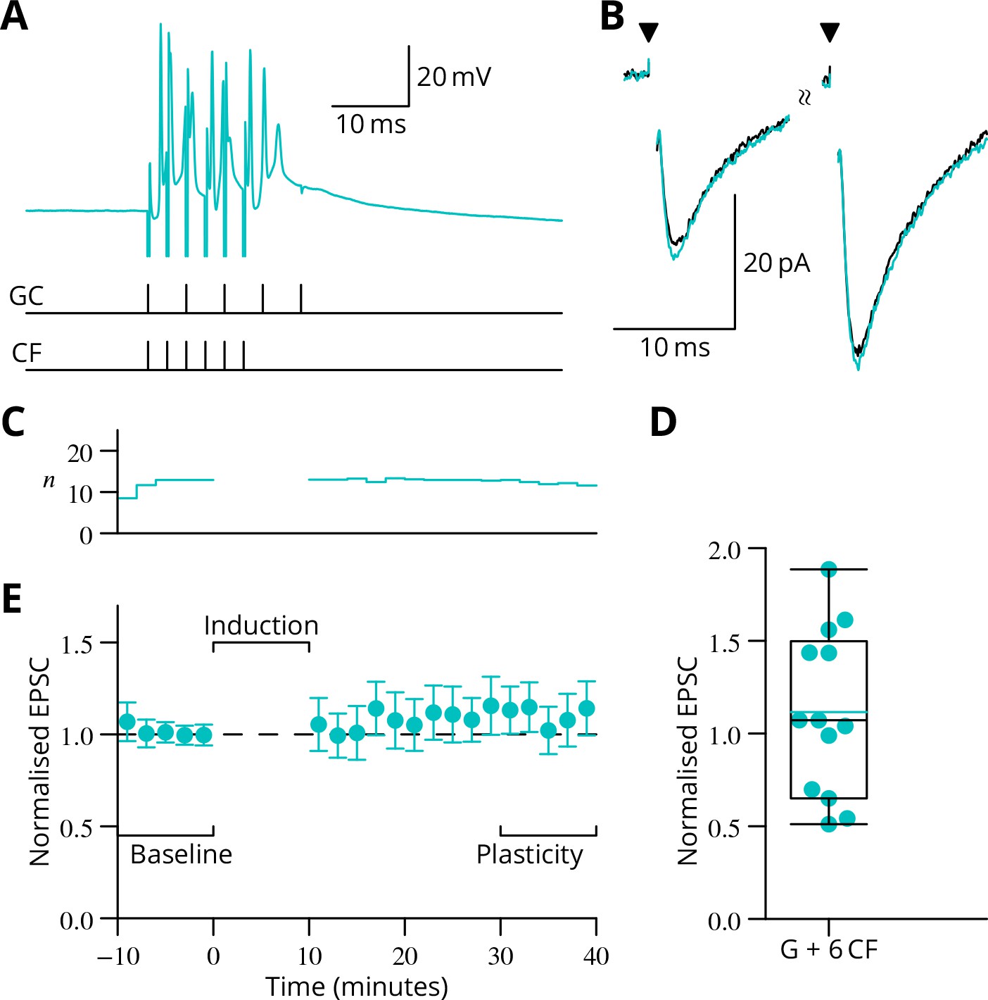
In complementary experiments, we examined the outcome of applying a burst of six climbing fibre stimuli simultaneously with the granule cell burst.

(A) Illustration of the induction protocol. (B) Specimen EPSCs before (*black*) and after (*cyan*) induction. (C) Time course of mean normalised EPSC amplitude ( $\pm$ SEM). (D) Scatter plot of plasticity ratios.

https://doi.org/10.7554/eLife.31599.008

Figure 7

Download asset Open asset

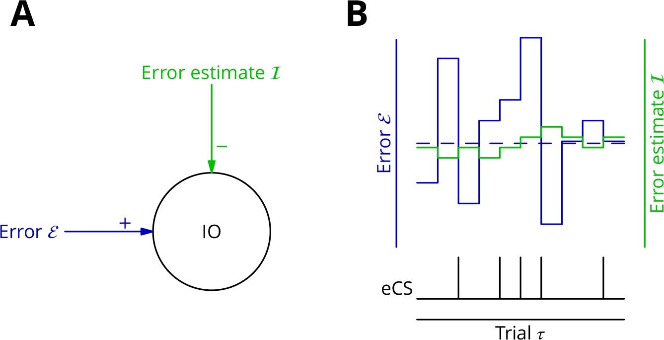
Adaptive tracking to cancel the mean error input to the inferior olive.

(A) The olive is assumed to receive an excitatory signal representing movement error $ℰ$ and an inhibitory input $ℐ$ from the nucleo-olivary neurones of the cerebellar nuclei. (B) The inputs to the inferior olive are represented in discrete time ( $τ$ )—each bar can be taken to represent a discrete movement realisation. The error (*blue*) varies about its average (*dashed blue line*) because perturbation complex spikes influence the movement and associated error randomly. The strength of the inhibition is shown by the *green* trace. When the excitatory error input exceeds the inhibition, an error complex spike is emitted (*bottom black trace*) and the inhibition is strengthened by plasticity, either directly or indirectly. In the converse situation and in the consequent absence of an error complex spike, the inhibition is weakened. In this way, the inhibition tracks the average error and the emission of an error complex spike signals an error exceeding the estimated average. Note that spontaneous perturbation complex spikes are omitted from this diagram.

https://doi.org/10.7554/eLife.31599.010

Figure 8

Download asset Open asset

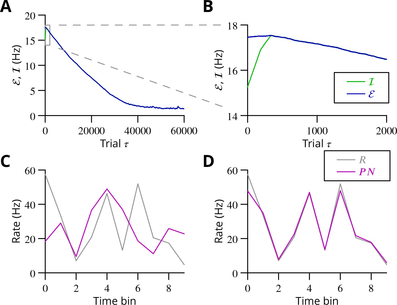
Simulated cerebellar learning by stochastic gradient descent with estimated global errors.

The total error ( $ℰ$ , *blue*) at the cerebellar nuclear output and the cancelling inhibition ( $ℐ$ , *green*) reaching the inferior olive are plotted as a function of trial number ( $τ$ ) in (A and B) for one of two interleaved patterns learnt in parallel. An approximately 10-fold reduction of error was obtained. It can be seen in A that the cancelling inhibition follows the error very closely over most of the learning time course. However, the zoom in B shows that there is no systematic reduction in error until the inhibition accurately cancels the mean error. (C) Initial firing profile of a typical cerebellar nuclear projection neurone ( $P N$ , *magenta*); the simulation represented 10 time bins with initially random frequency values per neurone, with a mean of 30 Hz. The target firing profile for the same neurone ( $R$ , *grey*) is also plotted. (D) At the end of the simulation, the firing profile closely matched the target.

https://doi.org/10.7554/eLife.31599.011

Figure 9

Download asset Open asset

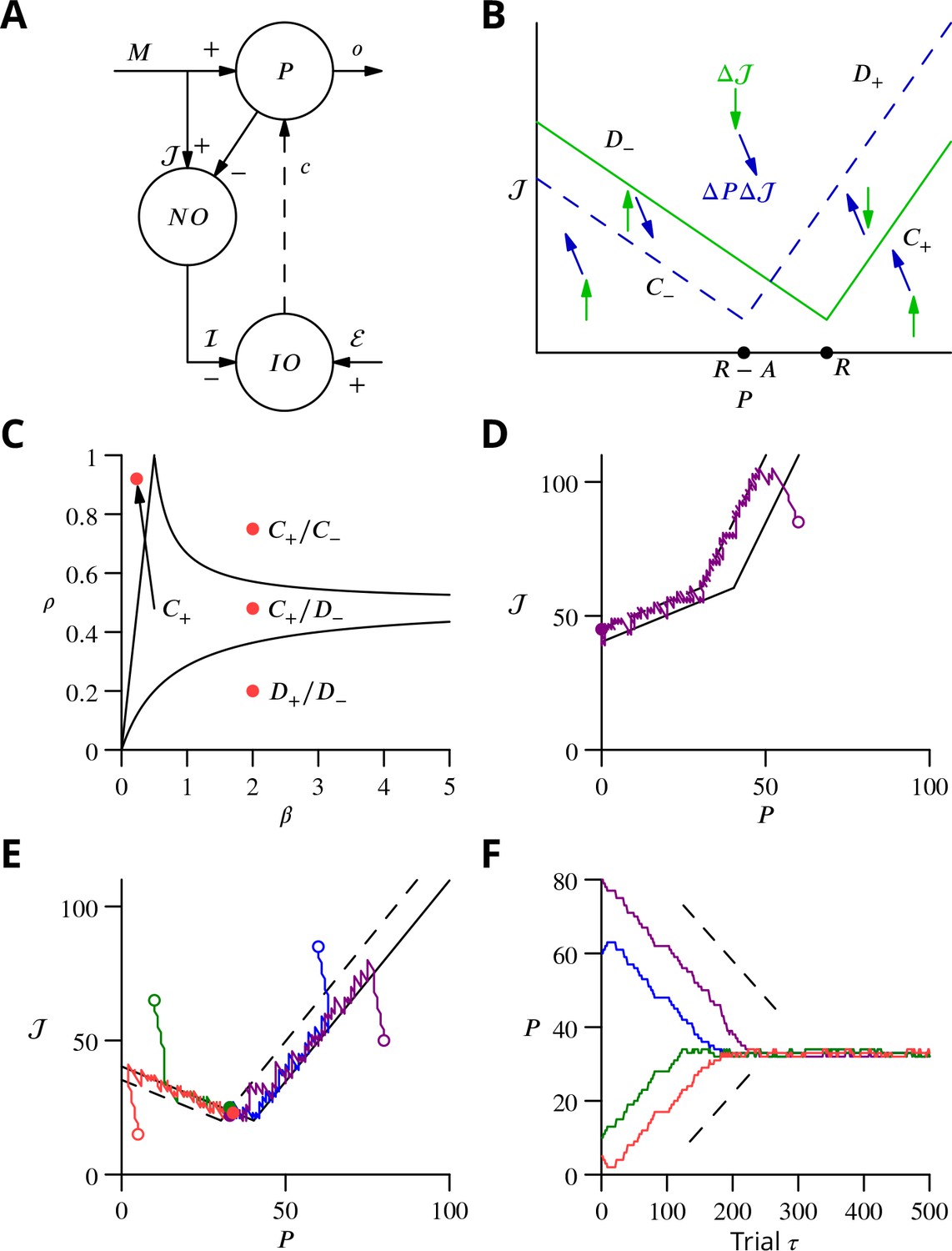
Single-cell convergence dynamics in a reduced version of the algorithm.

(A) Simplified circuitry implementing stochastic gradient descent with estimated global errors. Combined Purkinje cells/projection neurones (P) provide the output $o$ . These cells receive an excitatory plastic input from mossy fibres ( $M$ ). Mossy fibres also convey a plastic excitatory input $𝒥$ to the nucleo-olivary neurones (NO), which receive inhibitory inputs from the Purkinje cells and supply the inhibitory input $ℐ = {[𝒥 - q P]}_{+}$ to the inferior olive (IO). The inferior olive receives an excitatory error input $ℰ$ . The olivary neurones emit spikes that are transmitted to the P-cells via the climbing fibre $c$ . (B) Effects of plasticity on the simplified system in the plane defined by the P-cell rate $P$ (with optimum $R$ , perturbation $A$ ) and excitatory drive to the nucleo-olivary neurones $𝒥$ . Plastic updates of type $Δ P Δ 𝒥$ (*blue arrows*) and $Δ 𝒥$ (*green arrows*) are shown. The updates change sign on the line C (*dashed blue*) and D (*solid green*), respectively. Lines $C_{\pm}$ and $D_{\pm}$ delimit the ‘convergence corridors’. The diagram is drawn for the case $q < 1$ , in which $A$ , the perturbation of $P$ is larger than the perturbation $q A$ of $ℐ$ . (C) Parameters $β$ and $ρ$ determine along which lines the system converges to $R$ . The *red dot* in the $D_{+} / D_{-}$ region shows the parameter values used in panels E and F and also corresponds to the effective parameters of the perceptron simulation of Figure 10. The other *red dots* show the parameters used in the learning examples displayed in Appendix 1—figure 1. (D) When $q > 1$ , $C_{+}$ and $D_{-}$ do not cross and learning does not converge to the desired rate. After going down the $C_{+} / D_{+}$ corridor, the point $(P, 𝒥)$ continues along the $C_{-} / D_{-}$ corridor without stopping close to the desired target rate $R$ . *Open circle*, start point; *filled circle*, end point. (E) Dynamics in the $(P, 𝒥)$ plane for $ρ = 0.2$ and $β = 2$ ( $A = 10, Δ P = 1, Δ 𝒥 = 2, q = 0.5$ ). Trajectories (*coloured lines*) start from different initial conditions (*open circles*). *Open circles*, start points; *filled circles*, end points. (F) Time courses of $P$ as a function of trial $τ$ for the trajectories in C (*same colours*). *Dashed lines*: predicted rate of convergence (Appendix 1). All trajectories end up fluctuating around $P = R - A (q + 1) / 2$ , which is $R - 7.5$ with the chosen parameters. *Open circles*, start points; *filled circles*, end points.

https://doi.org/10.7554/eLife.31599.012

Figure 10

Download asset Open asset

Convergence and capacity for an analog perceptron.

(A) Convergence for a single learned pattern for stochastic gradient descent with estimated global errors (SGDEGE). Different lines (*thin grey lines*) correspond to distinct simulations. The linear decrease of the error ( $P - R$ ) predicted from the simplified model without zero-weight synapses is also shown (*dashed lines*). When learning increases the rate towards its target, the predicted convergence agrees well with the simulation. When learning decreases the rate towards its target, the predicted convergence is larger than observed because a fraction of synapses have zero weight. (B) Mean error vs. number of trials (always per pattern) for different numbers of patterns for SGDEGE with $q = 0.5$ . *Colours from black to red*: 50, 100, 200, 300, 350, 380, 385, 390, 395, 400, 410, 420, 450. (C) Mean error vs. number of trials when learning using the delta rule. The final error is zero when the number of patterns is below capacity (predicted to be 391 for these parameters), up to finite size effects. *Colours from black to blue*: same numbers of patterns as listed for B. (D) Mean error after $1 \times 10^{5}$ trials for the delta rule (*blue*) and for the SGDEGE with $q = 0$ (*cyan*), 0.25 (*green*), 0.5 (*red*), 0.75 (*magenta*), as a function of the number of patterns $p$ . The mean error diverges from its minimal value close to the theoretical capacity (*dashed line*) for both learning algorithms. (E) Dynamics of pattern learning in the $P - 𝒥$ or more precisely $(P - R) - (𝒥 - q P)$ plane below maximal capacity ( $p = 300$ ). The error ( $P - R$ ) corresponding to each pattern (*grey*) is reduced as it moves down its convergence corridor. The trajectory for a single specimen pattern is highlighted in *red*, while the endpoints of all trajectories are indicated by *salmon filled circles* but are all obscured at (0,0) by the *red filled circle* of the specimen trajectory. (F) Same as in E for a number of patterns above maximal capacity ( $p = 420$ ). After learning several patterns, rates remain far from their targets (*salmon filled circles*). The SGDEGE algorithm parameters used to generate this figure are $A = 2, Δ 𝒥 = 0.4, Δ P = 0.2, ρ = 0.2$ . The parameter $q = 0.5$ except in panel D where it is explicitly varied. The analog perceptron parameters are $P_{m a x} = 100, f = 0.2, N_{m} = 1000$ and the threshold $θ = 12.85$ with $γ = 1$ ).

https://doi.org/10.7554/eLife.31599.013

Figure 11

Download asset Open asset

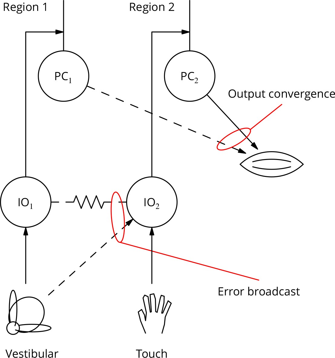
Diagram illustrating two possible solutions to the ‘bicycle problem’: how to use vestibular error information to guide learning of arm movements to ride a bicycle.

In the ‘output convergence’ solution, the outputs from cerebellar regions receiving different climbing fibre modalities converge onto a motor unit (represented by a muscle in the diagram). In the ‘error broadcast’ solution, error complex spikes are transmitted beyond their traditional receptive fields, either by divergent synaptic inputs and/or via the strong electrical coupling between inferior olivary neurones.

https://doi.org/10.7554/eLife.31599.014

Figure 12

Download asset Open asset

Diagram of the simulated network model.

The details are explained in the text.

https://doi.org/10.7554/eLife.31599.015

Appendix 1—figure 1

Download asset Open asset

Reduced model: different cases of stochastic gradient learning are illustrated, for the parameters marked by *solid red circles* in Figure 9C, except for the case already shown in Figure 9E and F.

(A) Dynamics in the $(P, 𝒥)$ plane for $ρ = 0.5$ and $β = 2$ ( $A = 10, Δ P = 1, Δ 𝒥 = 2$ ). Trajectories (*solid lines*) from different initial conditions (*open circles*) are represented in the $(P, 𝒥)$ plane. The trajectories converge by oscillating around $C_{+}$ in the $C_{+} / D_{+}$ ‘corridor’ and around $D_{-}$ in the $C_{-} / D_{-}$ ‘corridor’. Trajectory endings are marked by *filled circles*. (B) Time courses of $P (τ)$ with corresponding colours. The slope of convergence (*dotted lines*) predicted by Equation 32 and 33 agrees well with the observed convergence rate for $C_{+}$ while it is less accurate for $D_{-}$ when the assumption that the ‘corridor’ width is much greater than $Δ P$ and $Δ 𝒥$ does not hold. (**C, D**) Same graphs for $ρ = 0.75$ . The trajectories converge by oscillating around $C_{+}$ in the $C_{+} / D_{+}$ and around $C_{-}$ in the $C_{-} / D_{-}$ ‘corridor’. (**E, F**) Same graphs for $ρ = 0.75$ and $β = 0.25$ (i.e. $A = 2, Δ P = 1, Δ 𝒥 = 0.25$ ). The trajectories converge by oscillating around $C_{+}$ , which is the only attractive line.

https://doi.org/10.7554/eLife.31599.019

Tables

Table 1

Group data and statistical tests for plasticity outcomes.

In the upper half of the table, the ratios of EPSC amplitudes after/before induction are described and compared with a null hypothesis of no change (ratio = 1). The GP_ and GPE protocols both induced changes, while the control protocols (G_ _, G_E) did not. The bottom half of the table analyses differences of those ratios between protocols. The 95% confidence intervals (c.i.) were calculated using bootstrap methods, while the $p$ -values were calculated using a two-tailed Wilcoxon rank sum test. The p-values marked with an asterisk have been corrected for a two-stage analysis by a factor of 2 (Materials and methods).

https://doi.org/10.7554/eLife.31599.009

Comparison	Mean	95 % c.i.		$p$	$n$
GP_	1.40	1.26,	1.72	0.0001	15
GPE	0.53	0.45,	0.63	0.002	10
G_ _	0.97	0.78,	1.16	0.77	18
G_E	0.98	0.79,	1.24	0.60	15
GP_ vs G_ _	0.43	0.19,	0.74	0.021*
GPE vs G_E	−0.44	−0.72,	−0.24	0.0018*
GP_ vs G_E	0.42	0.14,	0.73	0.01*
GPE vs G_ _	−0.43	−0.65,	−0.22	0.008*
G_ _ vs G_E	0.01	−0.26,	0.32	0.93

Table 2

Parameters used in the simulation shown in Figure 12.

https://doi.org/10.7554/eLife.31599.016

Parameter	Symbol	Value
Sagittal extent	$S$	10
Lateral extent	$L$	40
Time bins per movement	$T$	10
Mossy fibres per sagittal position	$N$	2000
Maximum firing rate (all neurones)	$r_{m a x}$	300 Hz
pCS probability per cell per movement	$ρ$	0.03
Amplitude of Purkinje cell firing perturbation	$A$	2 Hz
Learning rate of $M \to P C$ synapses	$α_{w}$	0.02
Learning rate of $M \to N O$ synapses	$α_{v}$	0.0002
Mean Purkinje cell firing rate	${\bar{r}}_{P C}$	50 Hz
Mean firing rate for nuclear neurones	${\bar{r}}_{D}$	30 Hz
$M \to P N$ synaptic weight	$u_{(M \to P N)}$	2.4
$P C \to P N$ synaptic weight	$u_{(P C \to P N)}$	$-$ 0.06
$P C \to N O$ relative synaptic weight	$q$	0.5
Weight increment of $M \to P C$ drift (simple model)	$β_{w}$	0.002

Additional files

Transparent reporting form: https://doi.org/10.7554/eLife.31599.017
Download elife-31599-transrepform-v1.pdf

Download links

A two-part list of links to download the article, or parts of the article, in various formats.

Downloads (link to download the article as PDF)

Open citations (links to open the citations from this article in various online reference manager services)

Mendeley

Cite this article (links to download the citations from this article in formats compatible with various reference manager tools)

Guy Bouvier
Johnatan Aljadeff
Claudia Clopath
Célian Bimbard
Jonas Ranft
Antonin Blot
Jean-Pierre Nadal
Nicolas Brunel
Vincent Hakim
Boris Barbour

(2018)

Cerebellar learning using perturbations

eLife 7:e31599.

https://doi.org/10.7554/eLife.31599

Figures

The cerebellar circuitry and properties of Purkinje cells.

Analysis of cerebellar learning.

Predicted plasticity rules.

Simultaneous granule cell and climbing fibre activity induces LTP.

LTD requires simultaneous granule cell and climbing fibre activity closely followed by an additional complex spike.

Time course and amplitude of plasticity.

In complementary experiments, we examined the outcome of applying a burst of six climbing fibre stimuli simultaneously with the granule cell burst.

Adaptive tracking to cancel the mean error input to the inferior olive.

Simulated cerebellar learning by stochastic gradient descent with estimated global errors.

Single-cell convergence dynamics in a reduced version of the algorithm.

Convergence and capacity for an analog perceptron.

Diagram illustrating two possible solutions to the ‘bicycle problem’: how to use vestibular error information to guide learning of arm movements to ride a bicycle.

Diagram of the simulated network model.

Reduced model: different cases of stochastic gradient learning are illustrated, for the parameters marked by solid red circles in Figure 9C, except for the case already shown in Figure 9E and F.

Tables

Group data and statistical tests for plasticity outcomes.

Parameters used in the simulation shown in Figure 12.

Additional files

Transparent reporting form

Download links

Downloads (link to download the article as PDF)

Open citations (links to open the citations from this article in various online reference manager services)

Cite this article (links to download the citations from this article in formats compatible with various reference manager tools)

Be the first to read new articles from eLife

Share this article

Cite this article

The cerebellar circuitry and properties of Purkinje cells.

Analysis of cerebellar learning.

Predicted plasticity rules.

Simultaneous granule cell and climbing fibre activity induces LTP.

LTD requires simultaneous granule cell and climbing fibre activity closely followed by an additional complex spike.

Time course and amplitude of plasticity.

In complementary experiments, we examined the outcome of applying a burst of six climbing fibre stimuli simultaneously with the granule cell burst.

Adaptive tracking to cancel the mean error input to the inferior olive.

Simulated cerebellar learning by stochastic gradient descent with estimated global errors.

Single-cell convergence dynamics in a reduced version of the algorithm.

Convergence and capacity for an analog perceptron.

Diagram illustrating two possible solutions to the ‘bicycle problem’: how to use vestibular error information to guide learning of arm movements to ride a bicycle.

Diagram of the simulated network model.

Reduced model: different cases of stochastic gradient learning are illustrated, for the parameters marked by solid red circles in Figure 9C, except for the case already shown in Figure 9E and F.

Group data and statistical tests for plasticity outcomes.

Parameters used in the simulation shown in Figure 12.

Transparent reporting form

Downloads (link to download the article as PDF)

Open citations (links to open the citations from this article in various online reference manager services)

Cite this article (links to download the citations from this article in formats compatible with various reference manager tools)