Highly multiplexed immunofluorescence imaging of human tissues and tumors using t-CyCIF and conventional optical microscopes
- Harvard Medical School, United States
- Dana-Farber Cancer Institute, United States
- Broad Institute of MIT and Harvard, United States
- Harvard University, United States
- Brigham and Women’s Hospital, Harvard Medical School, United States
Figures
Figure 1 with 2 supplements
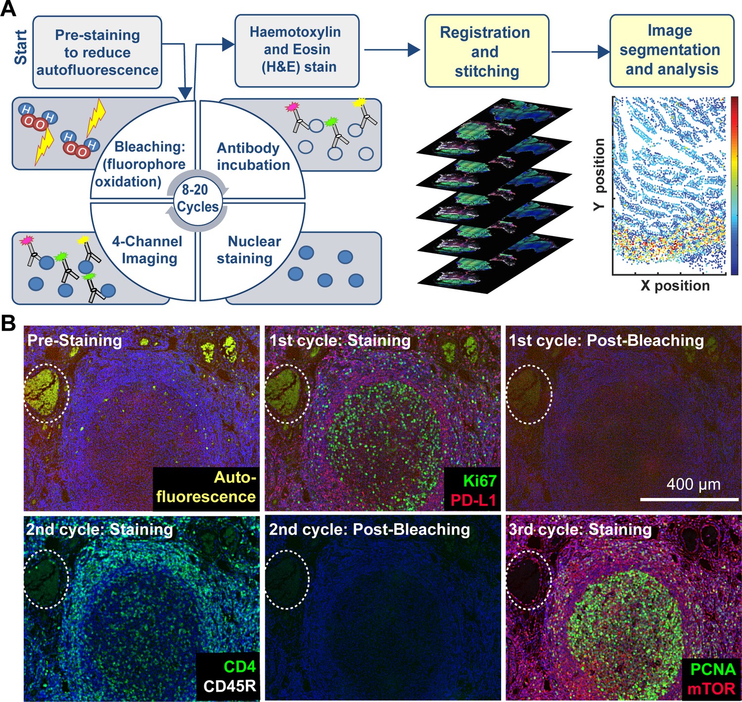
Steps in the t-CyCIF process.
(A) Schematic of the cyclic process whereby t-CyCIF images are assembled via multiple rounds of four-color imaging. (B) Image of human tonsil prior to pre-staining and then over the course of three rounds of t-CyCIF. The dashed circle highlights a region with auto-fluorescence in both green and red channels (used for Alexa-488 and Alexa-647, respectively) and corresponds to a strong background signal. With subsequent inactivation and staining cycles (three cycles shown here), this background signal becomes progressively less intense; the phenomenon of decreasing background signal and increasing signal-to-noise ratio as cycle number increases was observed in several staining settings (see also Figure 1—figure supplement 1).
Figure 1—figure supplement 1
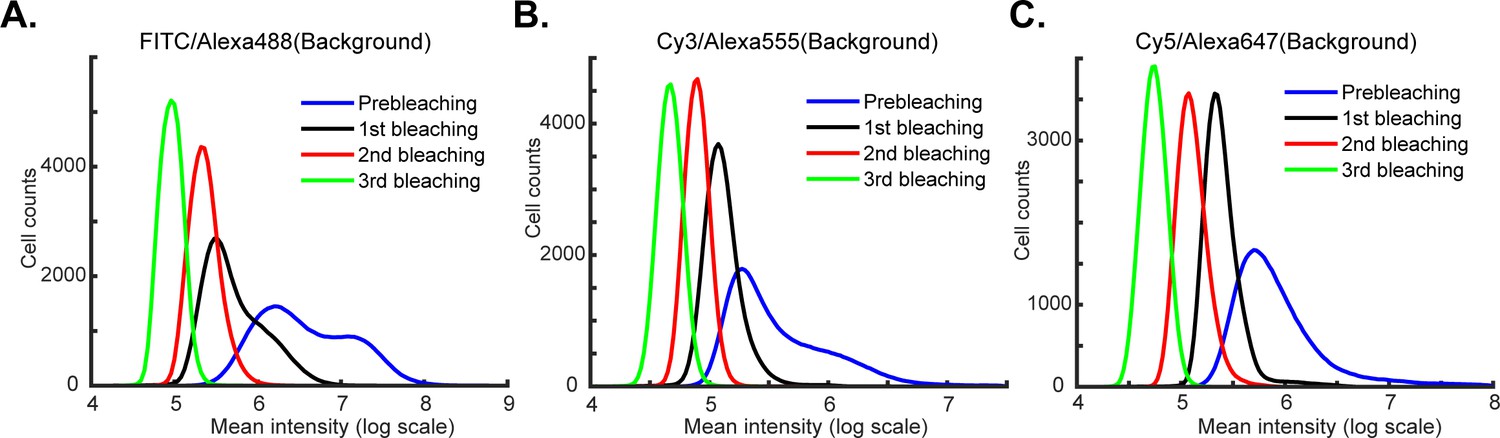
Reduction in background signal intensity with repeated cycles of bleaching.
(A–C) Intensity distributions for three fluorescence channels (FITC/Alexa-488, Cy3/Alexa-555 and Cy5/Alexa-647) prior to pre-bleaching (blue), and after 1, 2 or 3 cycles of bleaching (black, red and green lines, respectively). With increasing number of bleaching cycles, the background signal is reduced 10- to 100-fold.
Figure 1—figure supplement 2
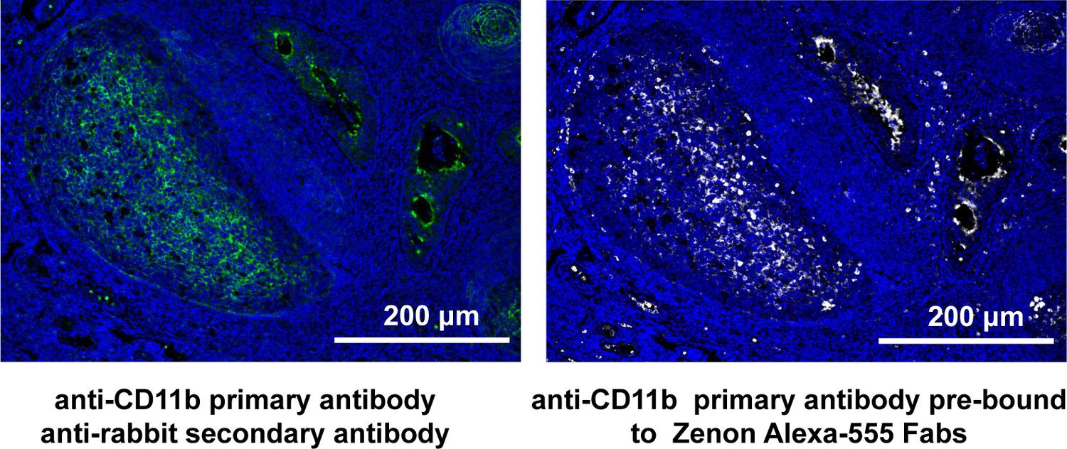
t-CyCIF using antibodies labelled with Zenon Alexa-555 Fab fragments.
A human tonsil specimen was stained with unconjugated anti-CD11b antibody and then with Alexa-488 conjugated anti-Rabbit secondary antibody (left) or with the same anti-CD11b antibody following incubation with Zenon Alexa-555 (ThermoFischer; right). The Zenon Fab fragments generate non-covalent immune complexes that ‘label’ the primary antibody in a manner that is stable to subsequent processing steps.
Figure 2 with 2 supplements
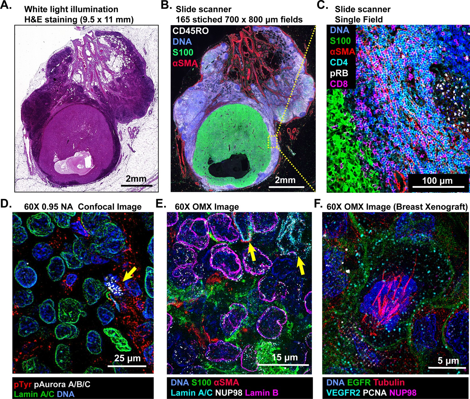
Multi-scale imaging of t-CyCIF specimens.
(A) Bright-field H&E image of a metastasectomy specimen that includes a large metastatic melanoma lesion and adjacent benign tissue. The H&E staining was performed after the same specimen had undergone t-CyCIF. (B) Representative t-CyCIF staining of the specimen shown in (A) stitched together using the Ashlar software from 165 successive CyteFinder fields using a 20X/0.8NA objective. (C) One field from (B) at the tumor-normal junction demonstrating staining for S100-postive malignant cells, α-SMA positive stroma, T lymphocytes (positive for CD3, CD4 and CD8), and the proliferation marker phospho-RB (pRB). (D) A melanoma tumor imaged on a GE INCell Analyzer 6000 confocal microscope to demonstrate sub-cellular and sub-organelle structures. This specimen was stained with phospho-Tyrosine (pTyr), Lamin A/C and p-Aurora A/B/C and imaged with a 60X/0.95NA objective. pTyr is localized in membrane in patches associated with receptor-tyrosine kinase, visible here as red punctate structures. Lamin A/C is a nuclear membrane protein that outlines the vicinity of the cell nucleus in this image. Aurora kinases A/B/C coordinate centromere and centrosome function and are visible in this image bound to chromosomes within a nucleus of a mitotic cell in prophase (yellow arrow). (E) Staining of a melanoma sample using the GE OMX Blaze structured illumination microscope with a 60X/1.42NA objective shows heterogeneity of structural proteins of the nucleus, including as Lamin B and Lamin A/C (indicated by yellow arrows) and part of the nuclear pore complex (NUP98) that measures ~120 nm in total size and indirectly allows the visualization of nuclear pores (indicated by non-continuous staining of NUP98). (F) Staining of a patient-derived mouse xenograft breast tumor using the OMX Blaze with a 60x/1.42NA objective shows a spindle in a mitotic cell (beta-tubulin in red) as well as vesicles staining positive for VEGFR2 (in cyan) and punctuate expression of the EGFR in the plasma membrane (in green).
Figure 2—figure supplement 1
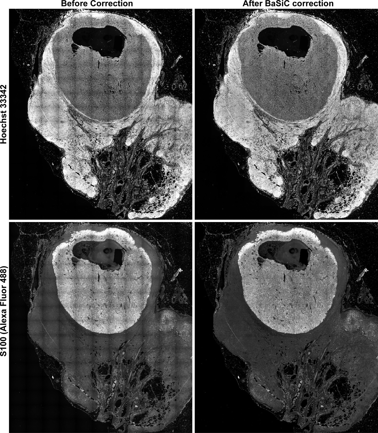
Flat-field and shading correction for stitched images.
A large melanoma specimen (same as shown specimen as in Figure 2A–B) was imaged with a 20X/0.8NA objective on a CyteFinder, and a total 165 frame images were assembled to one image using the ASHLAR algorithm. Representative channels (Hoechst 33342 and S100-Alexa-488) of the stitched images before (left) and after (right) correction for uneven illumination using the BaSiC algorithm (Peng et al., 2017) (see Materials and methods).
Figure 2—figure supplement 2

OMX super-resolution t-CyCIF images.
(A) Single-channel images for the composite image shown in Figure 2E. This melanoma sample was imaged using the GE OMX Blaze structured illumination microscope with 60X/1.42NA objectives. (B). Single-channel images for the composite image shown in Figure 2F. This breast cancer xenograft sample was also imaged using the OMX Blaze.
Figure 3
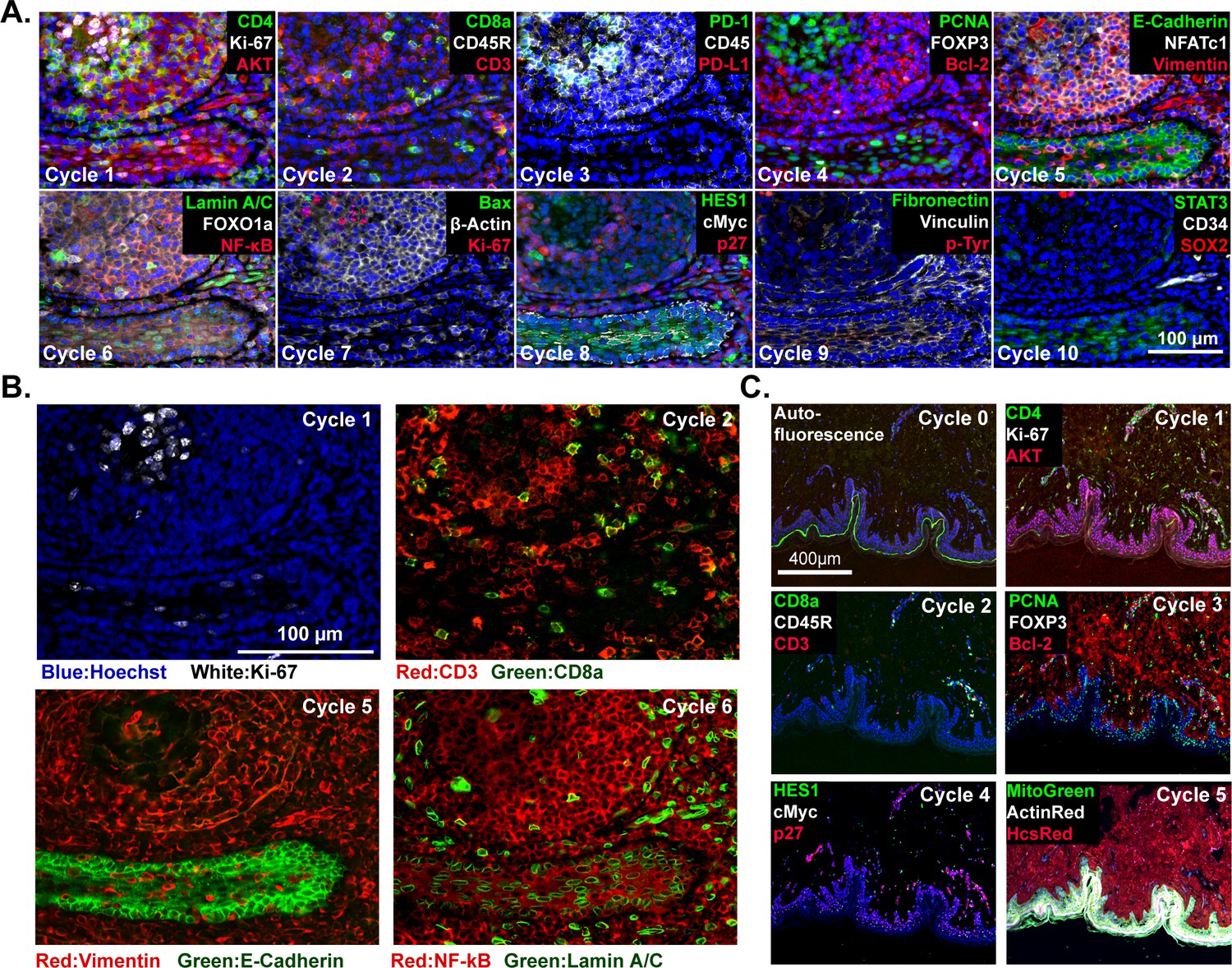
t-CyCIF imaging of normal tissues.
(A) Selected images of a tonsil specimen subjected to 10-cycle t-CyCIF to demonstrate tissue, cellular, and subcellular localization of tissue and immune markers (see Supplementary file 1 for a list of antibodies). (B) Selected cycles from (A) demonstrating sub-nuclear features (Ki67 staining, cycle 1), immune cell distribution (cycle 2), structural proteins (E-Cadherin and Vimentin, cycle 5) and nuclear vs. cytosolic localization of transcription factors (NF-kB, cycle 6). (C) Five-cycle t-CyCIF of human skin to show the tight localization of some auto-fluorescence signals (Cycle 0), the elimination of these signals after pre-staining (Cycle 1), and the dispersal of rare cell types within a complex layered tissue (see Supplementary file 1 for a list of the antibodies).
Figure 4 with 1 supplement
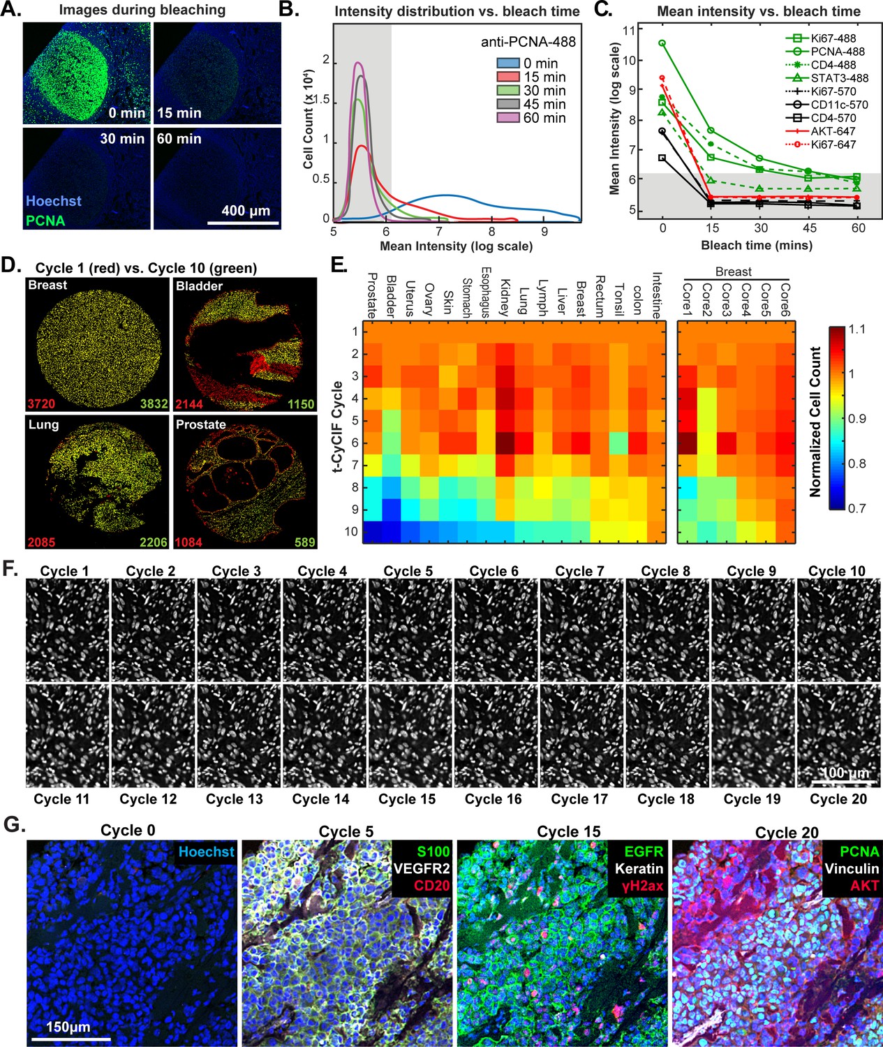
Efficacy of fluorophore inactivation and preservation of tissue integrity.
(A) Exemplary image of a human tonsil stained with PCNA-Alexa 488 that underwent 0, 15, 30 or 60 min of fluorophore inactivation. (B) Effect of bleaching duration on the distribution of anti-PCNA-Alexa 488 staining intensities for samples used in (A). The distribution is computed from mean values for the fluorescence intensities across all cells in the image that were successfully segmented. The gray band denotes the range of background florescence intensities (below 6.2 in log scale). (C) Effect of bleaching duration on mean intensity for nine antibodies conjugated to Alexa fluor 488, efluor 570 or Alexa fluor 647. Intensities were determined as in (B). The gray band denotes the range of background florescence intensities. (D) Impact of t-CyCIF cycle number on tissue integrity for four exemplary tissue cores. Nuclei present in the first cycle are labeled in red and those present after the 10th cycle are in green. The numbers at the bottom of the images represent nuclear counts in cycle 1 (red) and cycle 10 (green), respectively. (E) Impact of t-CyCIF cycle number on the integrity of a TMA containing 48 biopsies obtained from 16 different healthy and tumor tissues (see Materials and methods for TMA details) stained with 10 rounds of t-CyCIF. The number of nuclei remaining in each core was computed relative to the starting value; small fluctuations in cell count explain values > 1.0 and arise from errors in image segmentation. Data for six different breast cores is shown to the right. (F) Nuclear staining of a melanoma specimen subjected to 20 cycles of t-CyCIF emphasizes the preservation of tissue integrity (22 ± 4%). (G) Selected images of the specimen in (F) from cycles 0, 5, 15 and 20.
-
Figure 4—source data 1
Mean intensity versus bleach time for multiple antibodies (Figure 4C).
- https://doi.org/10.7554/eLife.31657.014
-
Figure 4—source data 2
Intensity distribution for single cells versus bleach time for one antibody (Figure 4B).
- https://doi.org/10.7554/eLife.31657.015
-
Figure 4—source data 3
Cell counts dependent on number of staining cycles (Figure 4E).
- https://doi.org/10.7554/eLife.31657.016
Figure 4—figure supplement 1
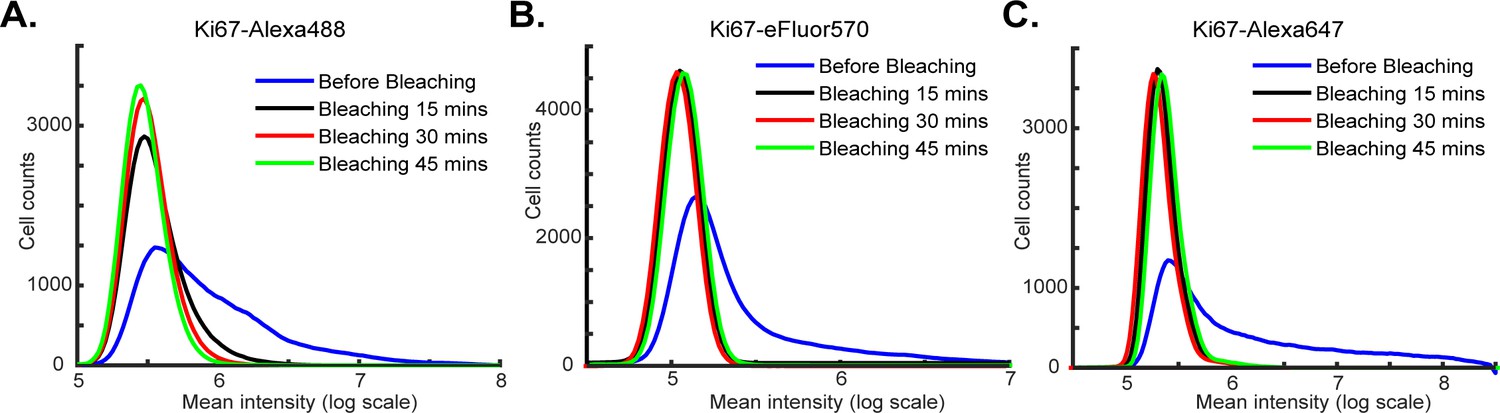
Impact of bleaching time on fluorophore inactivation.
Intensity distributions for specimens stained with an antibody against Ki67 coupled to the following fluorophores: (A) Alexa-488, (B) Alexa-570 and (C) Alexa-647 prior to bleaching (blue curves) and after 15, 30 or 45 min of bleaching (black, red and green curves respectively). The distributions were calculated from the average fluorescence intensities of single cells as determined after image segmentation.
Figure 5
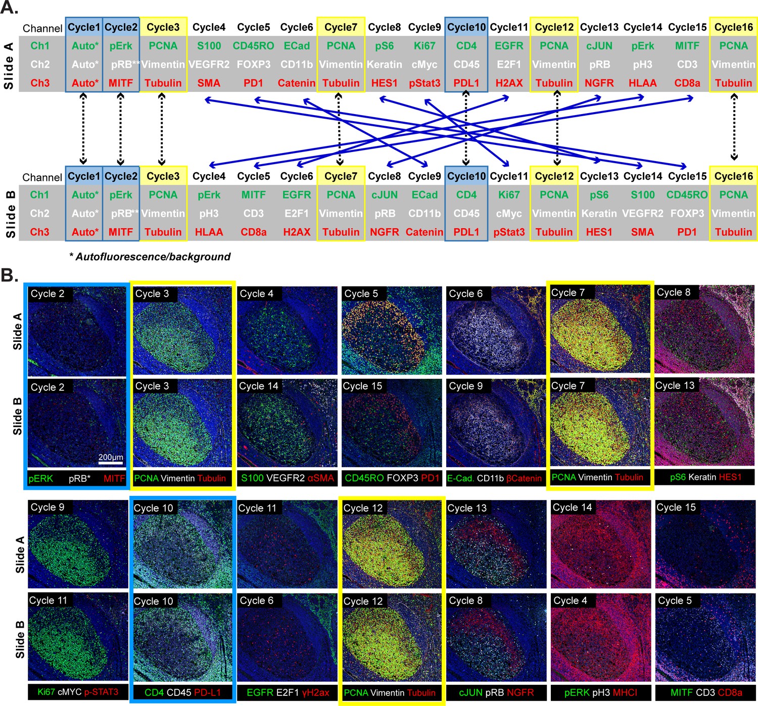
Design of a 16-cyle experiment used to assess the reliability of t-CyCIF data.
(A) t-CyCIF experiment involving two immediately adjacent tissue slices cut from the same block of tonsil tissue (Slide A and Slide B). The antibodies used in each cycle are shown (antibodies are described in Supplementary file 2). Highlighted in blue are cycles in which the same antibodies were used on slides A and B at the same time to assess reproducibility. Highlighted in yellow are cycles in which antibodies targeting PCNA, Vimentin and Tubulin were used repeatedly on both slides A and B to assess repeatability. Blue arrows connecting Slides A and B show how antibodies were swapped among cycles. (B) Representative images of Slide A (top panels) and Slide B specimens (bottom panels) after each t-CyCIF cycle. The color coding highlighting specific cycles is the same as in A.
Figure 6 with 1 supplement
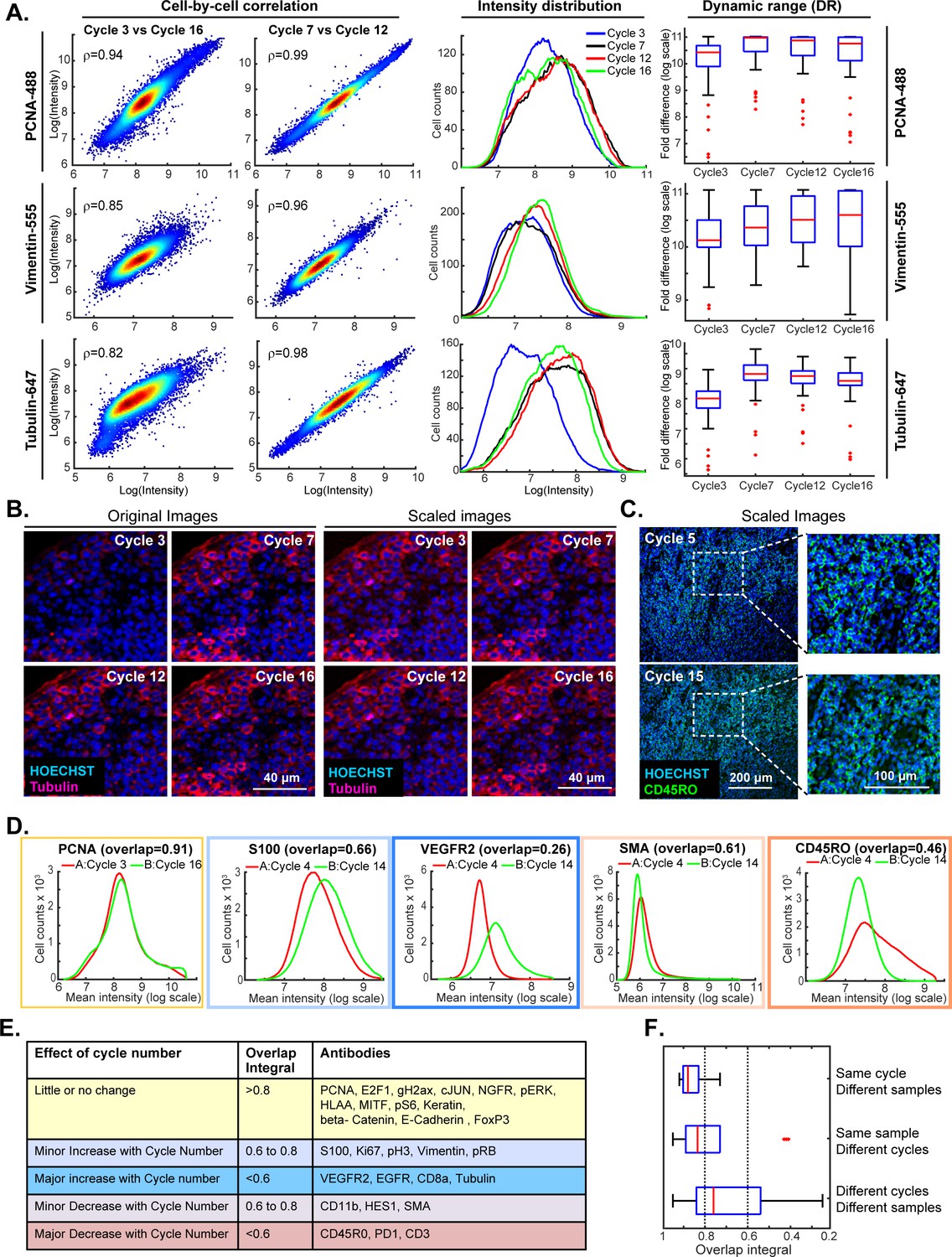
Impact of cycle number on repeatability, reproducibility and strength of t-CyCIF immuno-staining.
(A) Plots on left: comparison of staining intensity for anti-PCNA Alexa 488 (top), anti-vimentin Alexa 555 (middle) and anti-tubulin Alexa 647 (bottom) in cycle 3 vs. 16 and cycle 7 vs. 12 of the 16-cycle t-CyCIF experiment show in Figure 5. Intensity values were integrated across whole cells and the comparison is made on a cell-by-cell basis. Spearman’s correlation coefficients are shown. Plots in middle: intensity distributions at cycles 3 (blue), 7 (yellow), 12 (red) and 16 (green); intensity values were integrated across whole cells to construct the distribution. Box plots to right: estimated dynamic range at four cycle numbers 3, 7, 12, 16. Red lines denote median intensity values (across 56 frames), boxes denote the upper and lower quartiles, whiskers indicate values outside the upper/lower quartile within 1.5 standard deviations, and red dots represent outliers. (B) Representative images showing anti-tubulin Alexa 647 staining at four t-CyCIF cycles; original images are shown on the left (representing the same exposure time and approximately the same illumination) and images scaled by histogram equalization to similar intensity ranges are shown on the right. (C) Image for anti-CD45RO-Alexa 555 at cycles 5 and 15 scaled to similar intensity ranges as described in (B); the dynamic range (DR) of the cycle 15 image is ~3.3 fold lower than that of the Cycle 5 image, but shows similar morphology. (D) Intensity distributions for selected antibodies that were used in different cycles on Slides A and B. Colors denote the degree of concordance between the slides ranging from high (overlap >0.8 in yellow; PCNA), slightly increased or decreased with increasing cycle (overlap 0.6 to 0.8 in light blue or light red; S100 and SMA) or substantially increased or decreased (overlap <0.6 in red or blue; VEGFR2 and CD45RO). (E) Summary of effects of cycle number on antibody staining based on the degree of overlap in intensity distributions (the overlap integral); color coding is the same as in (D). (F) Effect of cycle number and specimen identity on overlap integrals for all antibodies and all cycles assayed. The red line denotes the median intensity value, boxes denote the upper/lower quartiles, and whiskers indicate values outside the upper/lower quartile and within 1.5 standard deviations, and red dots represent outliers. All the numeric data in Figures 5 and 6 are available in a Jupyter notebook; see Code Availability section of Materials and methods for details.
-
Figure 6—source data 1
Single-cell intensity data used in Figure 6.
- https://doi.org/10.7554/eLife.31657.020
Figure 6—figure supplement 1
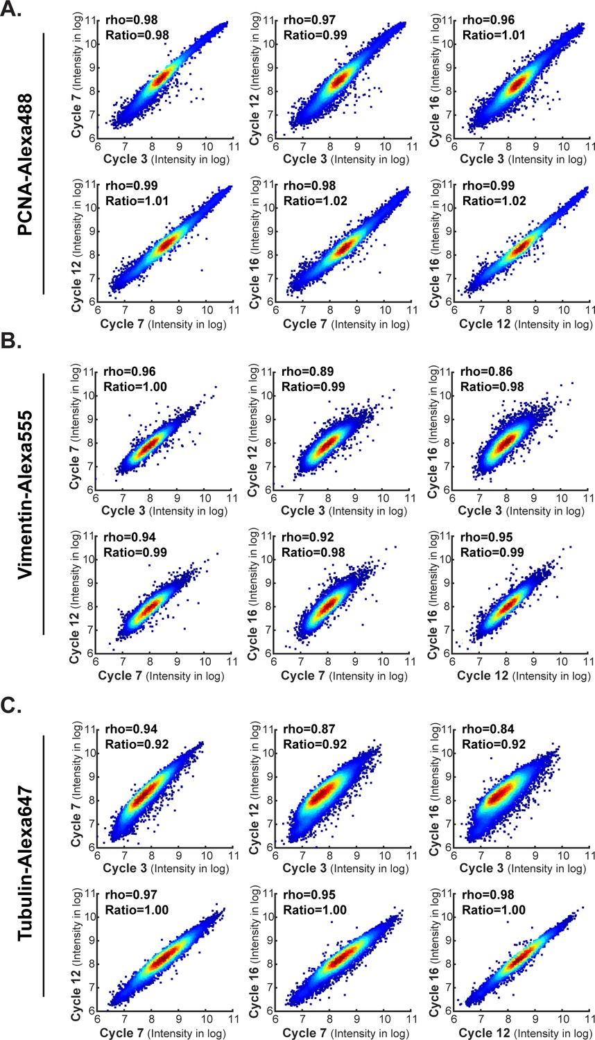
Comparison of staining intensities across different cycles at a single-cell level.
Images come from the antibody-swap and repeat experiment showing in Figures 5 and 6. Comparison of single-cell level intensities for (A) PCNA Alexa-488, (B) Vimentin Alexa-555 and (C) Tubulin Alexa-647 stained in four different cycles (cycle 3, 7, 12 and16). For any given cycle pair, single-cell intensities density plots are shown. Spearman’s correlation coefficients (rho) and the mean intensity ratios between two cycles are shown.
Figure 7 with 1 supplement
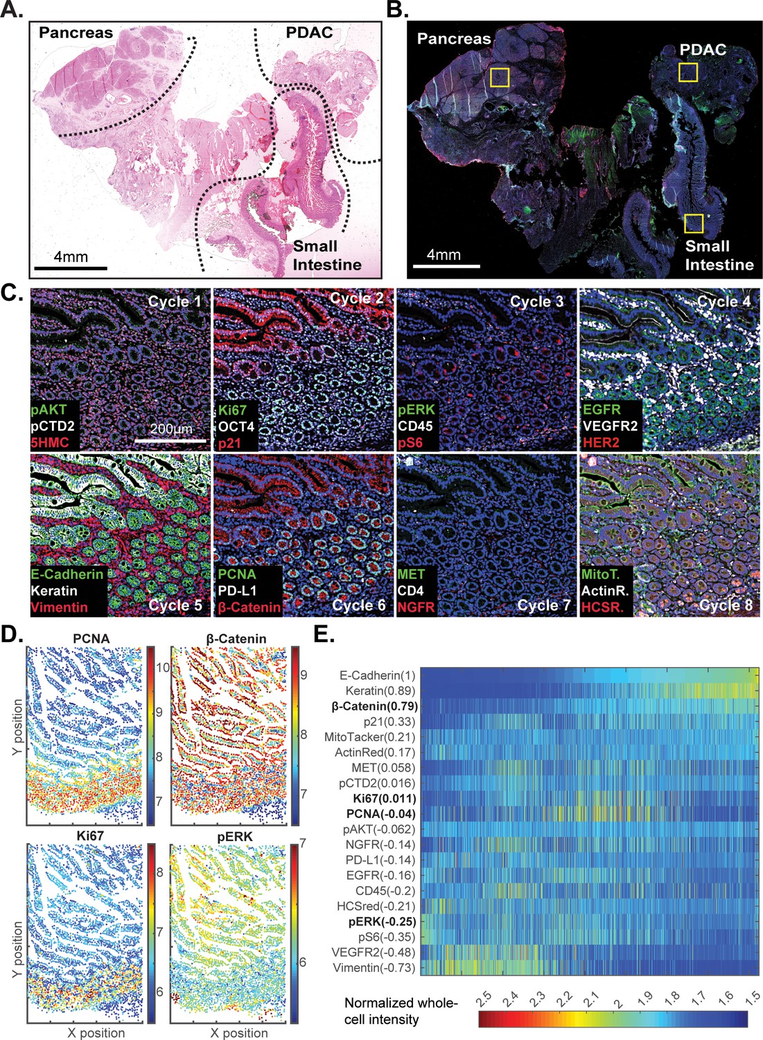
t-CyCIF of a large resection specimen from a patient with pancreatic cancer.
(A) H&E staining of pancreatic ductal adenocarcinoma (PDAC) resection specimen that includes portions of cancer and non-malignant pancreatic tissue and small intestine. (B) The entire sample comprising 143 stitched 10X fields of view is shown. Fields that were used for downstream analysis are highlighted by yellow boxes. (C) A representative field of normal intestine across 8 t-CyCIF rounds; see Supplementary file 3 for a list of antibodies. (D) Segmentation data for four antibodies; the color indicates fluorescence intensity (blue = low, red = high). (E) Quantitative single-cell signal intensities of 24 proteins (rows) measured in ~4×10³ cells (columns) from panel (C). The Pearson correlation coefficient for each measured protein with E-cadherin (at a single-cell level) is shown numerically. Known dichotomies are evident such as anti-correlated expression of epithelial (E-Cadherin) and mesenchymal (Vimentin) proteins. Proteins highlighted in red are further analyzed in Figure 8.
-
Figure 7—source data 1
Single-cell intensity data used in Figure 7E.
- https://doi.org/10.7554/eLife.31657.023
-
Figure 7—source data 2
- https://doi.org/10.7554/eLife.31657.024
Figure 7—figure supplement 1
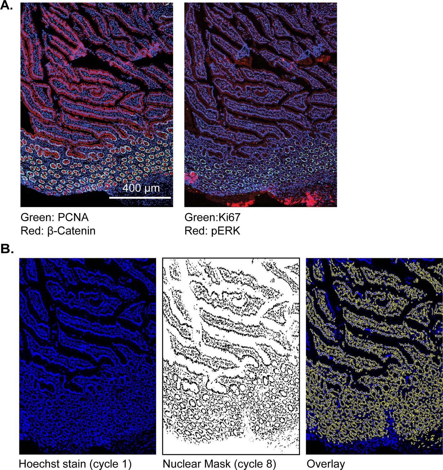
t-CyCIF for examining large resection specimens of a human pancreatic cancer.
(A) Representative frame of small intestine from the PDAC resection shown in Figure 7 with images for PCNA, beta-catenin, Ki67 and pERk shown. These frames correspond to the segmented panels shown in 7D. (B) Creation of nuclear masks following identification of nuclei. Left panel: Hoechst image from t-CyCIF cycle one on the PDAC resection sample; middle panel: a binarized nuclear mask from cycle 8 (the final cycle in this t-CyCIF experiment); right panel: the overlay image of Hoechst stain (blue) and the cycle eight nuclear mask (yellow). The final cycle is used to create the mask used in this analysis so that the same cells can be tracked through all t-CyCIF cycles despite ~15% overall cell loss by cycle 8. Thus, regions in the overlay that show up in blue correspond in most cases to cells that are lost in the course of t-CyCIF and not to failure to identity and segment cells correctly.
Figure 8
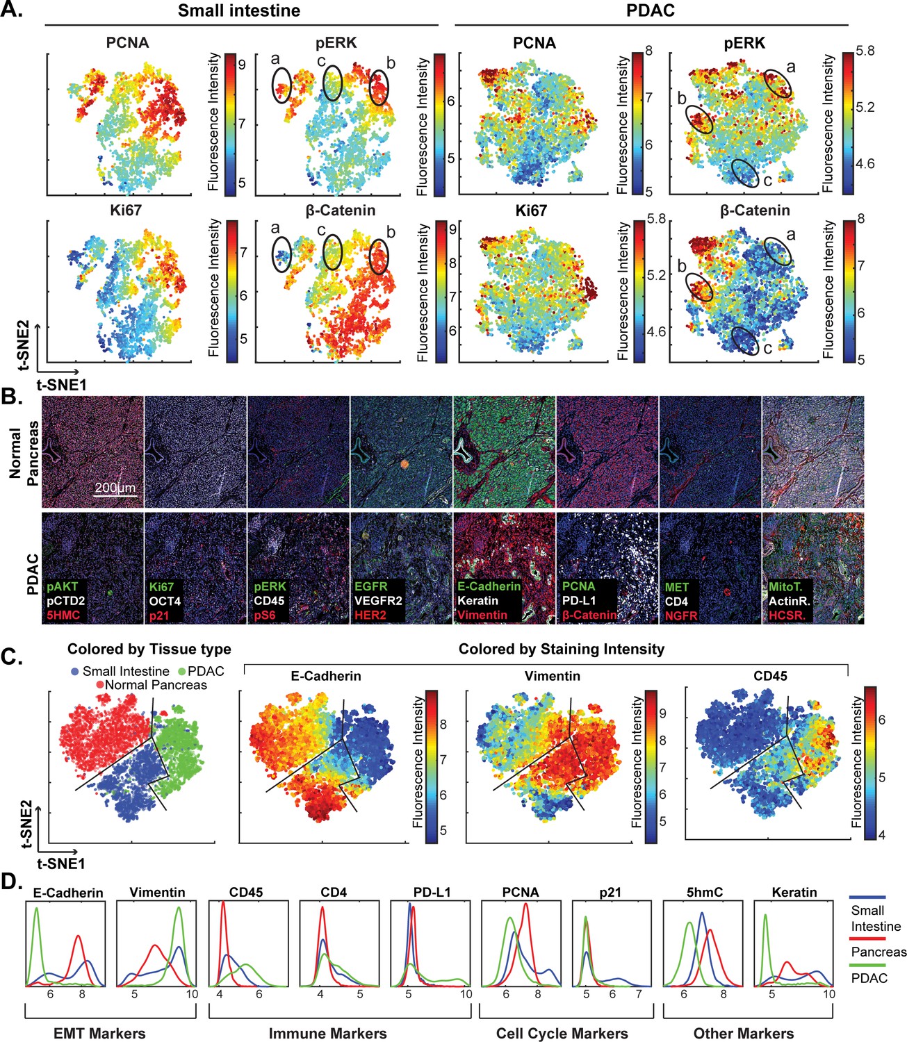
High-dimensional single-cell analysis of human pancreatic cancer sample with t-CyCIF.
(A) t-SNE plots of cells derived from small intestine (left) or the PDAC region (right) of the specimen shown in Figure 7 with the fluorescence intensities for markers of proliferation (PCNA and Ki67) and signaling (pERK and β-catenin) overlaid on the plots as heat maps. In both tissue types, there exists substantial heterogeneity: circled areas indicate the relationship between pERK and β-catenin levels in cells and represent positive (‘a’), negative (‘b’) or no association (‘c’) between these markers. (B) Representative frames of normal pancreas and pancreatic ductal adenocarcinoma from the 8-cycle t-CyCIF staining of the same resection specimen from Figure 7. (C) t-SNE representation and clustering of single cells from normal pancreatic tissue (red), small intestine (blue) and pancreatic cancer (green). Projected onto the origin of each cell in t-SNE space are intensity measures for selected markers demonstrating distinct staining patterns. (D) Fluorescence intensity distributions for selected markers in small intestine, pancreas and PDAC.
-
Figure 8—source data 1
Single-cell data in FCS format (Figure 8C–E).
- https://doi.org/10.7554/eLife.31657.026
Figure 9 with 1 supplement
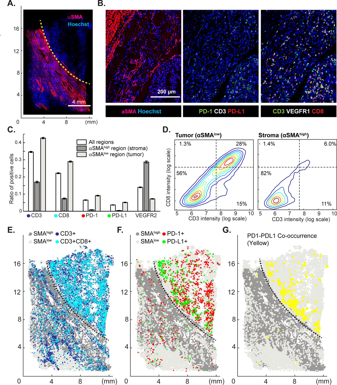
Spatial distribution of immune infiltrates and checkpoint proteins.
(A) Low-magnification image of a clear cell renal cancer subjected to 12-cycle t-CyCIF (see Supplementary file 4 for a list of antibodies). Regions high in α-smooth muscle actin (α-SMA) correspond to stromal components of the tumor, those low in α-SMA represent regions enriched for malignant cells. (B) Representative images from selected t-CyCIF channels are shown. (C) Quantitative assessment of total lymphocytic cell infiltrates (CD3+ cells), CD8+ T lymphocytes, cells expressing PD-1 or its ligand PD-L1 or the VEGFR2 for the entire tumor or for α-SMAhigh and α-SMAlow regions. VEGFR2 is a protein primarily expressed in endothelial cells and is targeted in the treatment of renal cell cancer. The error bars represent the S.E.M. derived from 100 rounds of bootstrapping. (D) Density plot for CD3 and CD8 expression on single cells in the tumor (left) or stromal domains (right). (E) Centroids of CD3+ or CD3+CD8+ cells in blue or dark blue as well as cells staining as SMAhigh or SMAlow (gray and light-gray, respectively) used to define the stromal and tumor regions. (F) Centroids of PD-1+ and PD-L1+ cells are shown in red and green, respectively. (G) Results of a K-nearest neighbor algorithm used to compute areas in which PD-1+ and PD-L1+ cells lie within ~10 µm of each other and with high spatial density (in yellow) and thus, are potentially positioned to interact at a molecular level.
-
Figure 9—source data 1
Immune cell counts from bootstrapping in tumor and stroma regions (Figure 9C).
- https://doi.org/10.7554/eLife.31657.029
-
Figure 9—source data 2
Single-cell intensity data used in Figure 9.
- https://doi.org/10.7554/eLife.31657.030
Figure 9—figure supplement 1
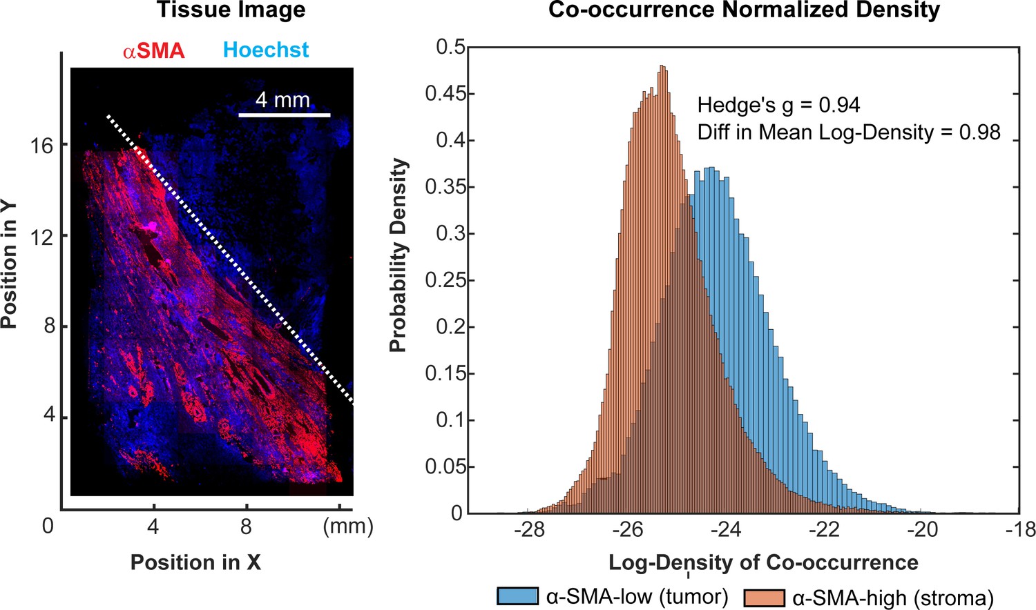
Spatial analysis of PD-1 and PD-L1 expressing cells.
This figure is relevant to the t-CyCIF study on a clear cell cancer shown in Figure 9. To compare co-localization of PD-1 and PD-L1 in tumor vs stroma, we computed the probability that PD1+ and PDL1+ cells would co-occur within a radius of ~10 um, normalizing for the difference in the total number of PD1+ and PDL1+ cells in the two tissue regions. We interpret the spatial density of PD1+ or PDL1+ cells at each point in space as proportional to the probability of their occurring there (see Figure 9E–F). The co-occurrence density at a point (Figure 9G) is therefore the product of the spatial densities for PD1+ or PDL1 +cells at that point. For simplicity, regions corresponding to tumor and stroma regions were defined by a diagonal line that separated the upper-right and lower-left regions of the tissue; this corresponded closely to α-SMA-low (tumor) and α-SMA-high (tumor) domains (left panel). We found an We found an e^(0.98)=2.7 fold difference in the distributions of co-occurrence densities between the two regions, representing an effect size of 0.94 as measured by Hedge's g; this represents a significant and potentially meaningful fold-change (right panel).
Figure 10 with 1 supplement
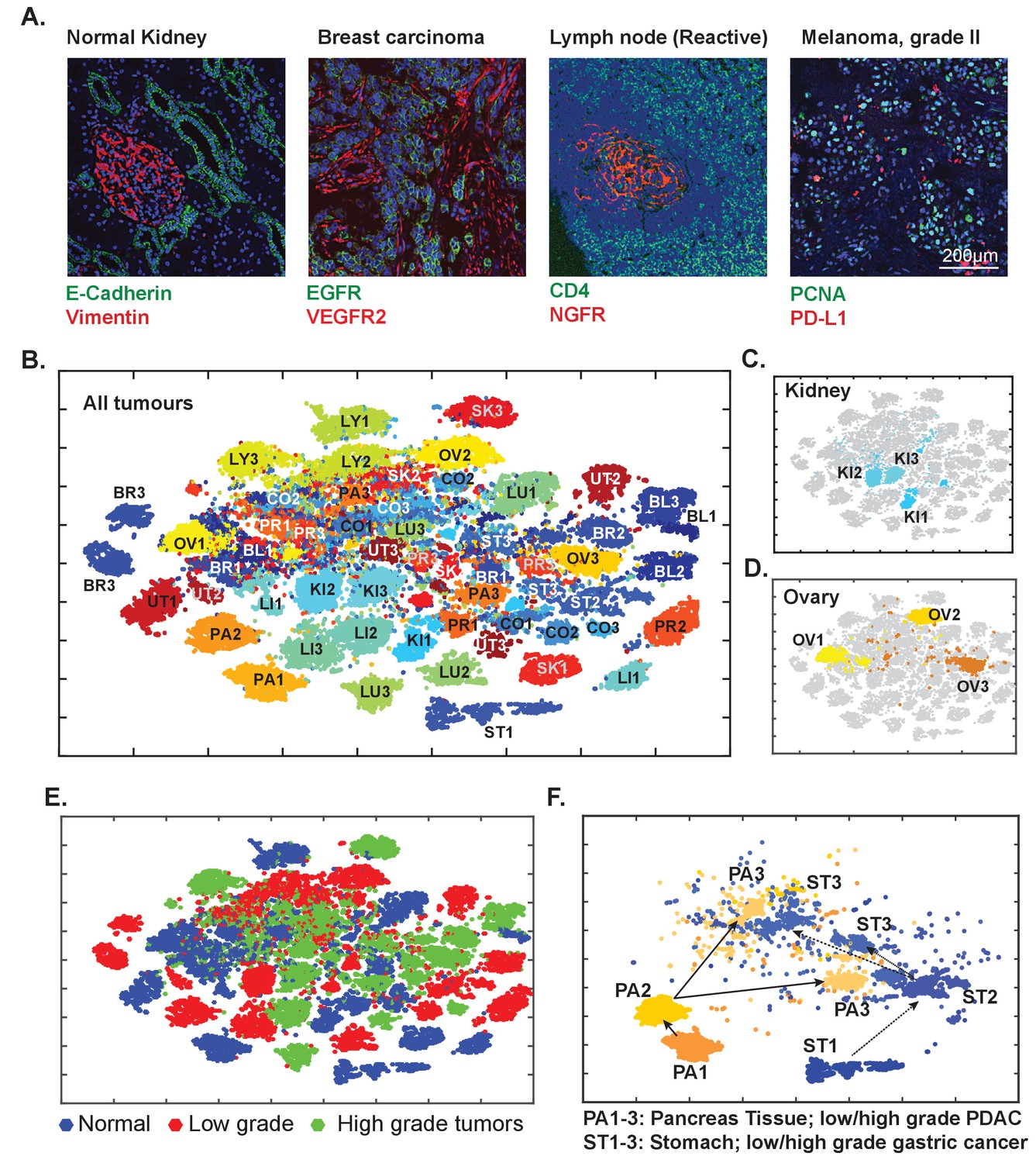
Eight-cycle t-CyCIF of a tissue microarray (TMA) including 13 normal tissues and corresponding tumor types.
The TMA includes normal tissue types, and corresponding high- and low-grade tumors, for a total of 39 specimens (see Supplementary file 3 for antibodies and Supplementary file 5 for specifications of the TMA). (A) Selected images of different tissues illustrating the quality of t-CyCIF images (additional examples shown in Figure 9—figure supplement 1; full data available online at www.cycif.org). (B) t-SNE plot of single-cell intensities of all 39 cores; data were analyzed using the CYT package (see Materials and methods). Tissues of origin and corresponding malignant lesions were labeled as follows: BL, bladder cancer; BR, breast cancer CO, Colorectal adenocarcinoma, KI, clear cell renal cancer, LI, hepatocellular carcinoma, LU, lung adenocarcinoma, LY, lymphoma, OV, high-grade serous adenocarcinoma of the ovary, PA, pancreatic ductal adenocarcinoma, PR, prostate adenocarcinoma, UT, uterine cancer, SK, skin cancer (melanoma), ST, stomach (gastric) cancer. Numbers refer to sample type; ‘1’ to normal tissue, ‘2’ to -grade tumors and ‘3’ to high-grade tumors. (C) Detail from panel B of normal kidney tissue (KI1) a low-grade tumor (KI2) and a high-grade tumor (KI3) (D) Detail from panel B of normal ovary (OV1) low-grade tumor (OV2) and high-grade tumor (OV3). (E) t-SNE plot from Panel B coded to show the distributions of all normal, low-grade and high-grade tumors. (F) tSNE clustering of normal pancreas (PA1) and pancreatic cancers (low-grade, PA2, and high-grade, PA3) and normal stomach (ST1) and gastric cancers (ST2 and ST3, respectively) showing intermingling of high-grade cells.
-
Figure 10—source data 1
Single-cell intensity data used in Figure 10.
- https://doi.org/10.7554/eLife.31657.033
Figure 10—figure supplement 1
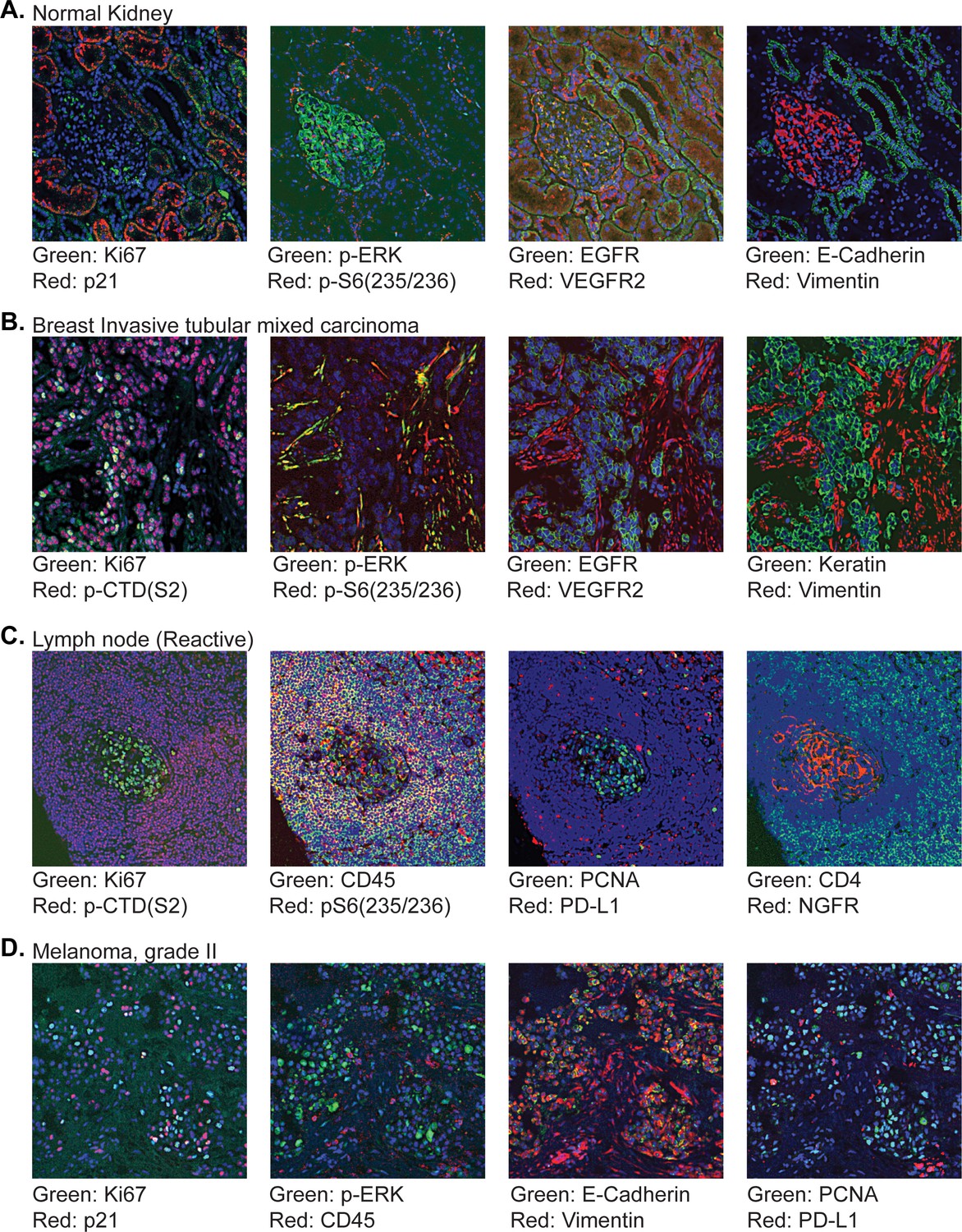
Gallery of exemplary tissues imaged on the TMA described in Figure 10.
Gallery of exemplary tissues imaged on the TMA described in Figure 10.
Figure 11
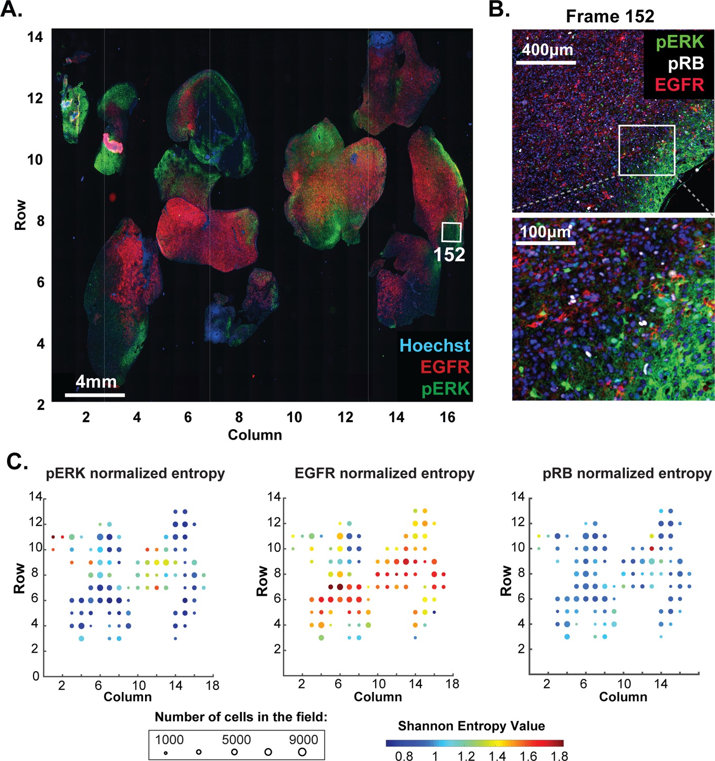
Molecular heterogeneity in a single GBM tumor.
(A) Representative low-magnification image of a GBM specimen generated from 221 stitched 10X frames; the sample was subjected to 10 rounds of t-CyCIF using antibodies listed in Supplementary file 6. (B) Magnification of frame 152 (whose position is marked with a white box in panel A) showing staining of pERK, pRB and EGFR; lower panel shows a further magnification to allow single cells to be identified. (C) Normalized Shannon entropy of each of 221 fields of view to determine the extent of variability in signal intensity for 1000 cells randomly selected from that field for each of the antibodies shown. The size of the circles denotes the number of cells in the field and the color represents the value of the normalized Shannon entropy (data are shown only for those fields with more than 1000 cells; see Materials and methods for details).
-
Figure 11—source data 1
Normalized entropy data shown in Figure 11C.
- https://doi.org/10.7554/eLife.31657.035
-
Figure 11—source data 2
- https://doi.org/10.7554/eLife.31657.036
Figure 12 with 2 supplements
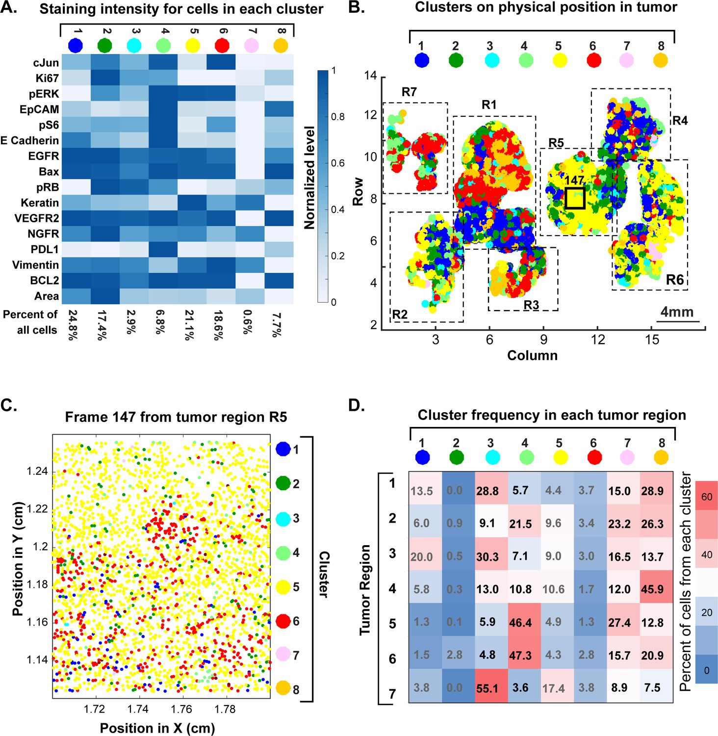
Spatial distribution of molecular phenotypes in a single GBM.
(A) Clustering of intensity values for 30 antibodies in a 10-cycle t-CyCIF analysis integrated over each whole cell based on images shown in Figure 11. Intensity values were clustered using expected-maximization with Gaussian mixtures (EMGM), yielding eight clusters, of which four clusters accounted for the majority of cells. The intensity scale shows the average level for each intensity feature in that cluster. The number of cells in the cluster is shown as a percentage of all cells in the tumor (bottom of panel). An analogous analysis is shown for 12 clusters in Figure 12—figure supplement 2. (B) EMGM clusters (in color code) mapped back to the positions of individual cells in the tumor. The coordinate system is the same as in Figure 11A. The positions of seven macroscopic regions (R1-R7) representing distinct lobes of the tumor are also shown. (C) Magnified view of Frame 147 from region R5 with EMGM cluster assignment for each cell in the frame; dots represent the centroids of single cells. (D) The proportional representation of EMGM clusters in each tumor region as defined in panel (B).
-
Figure 12—source data 1
Ratios of EMGM clusters in different regions of a GBM (Figure 12D).
- https://doi.org/10.7554/eLife.31657.040
Figure 12—figure supplement 1
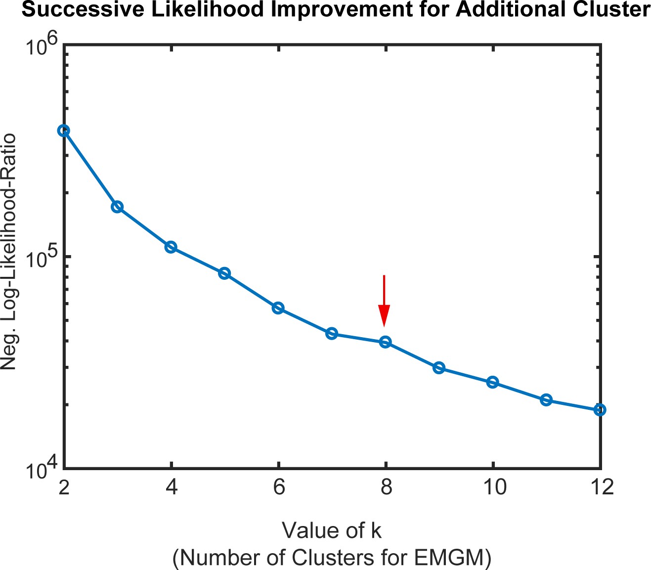
Determination of cluster number for semi-supervised clustering using expectation–maximization Gaussian mixture (EMGM) modeling.
To determine an appropriate number of clusters (k) for analysis of the GBM tumor shown in Figure 12 we determined negative log-likelihood-ratio for various values of k. Due to the large sample size, likelihood-ratio tests were not helpful in choosing k. Thus, for each choice of cluster number n, the likelihood-ratio was calculated for a Gaussian mixture model with n = k-1 and with n = k and the ratio then plotted relative to k. The EMGM algorithm was initialized 30 times for each value of k and it converged in all instances. The inflection at k = 8 (red arrow) suggested that inclusion of additional clusters (k > 8) explains a smaller, distinct source of variation in the data. The plot is shown on a logarithmic scale to better visualize the range of the log-likelihood ratios, and should not be confused with the logarithm already applied to the likelihood ratios themselves.
Figure 12—figure supplement 2
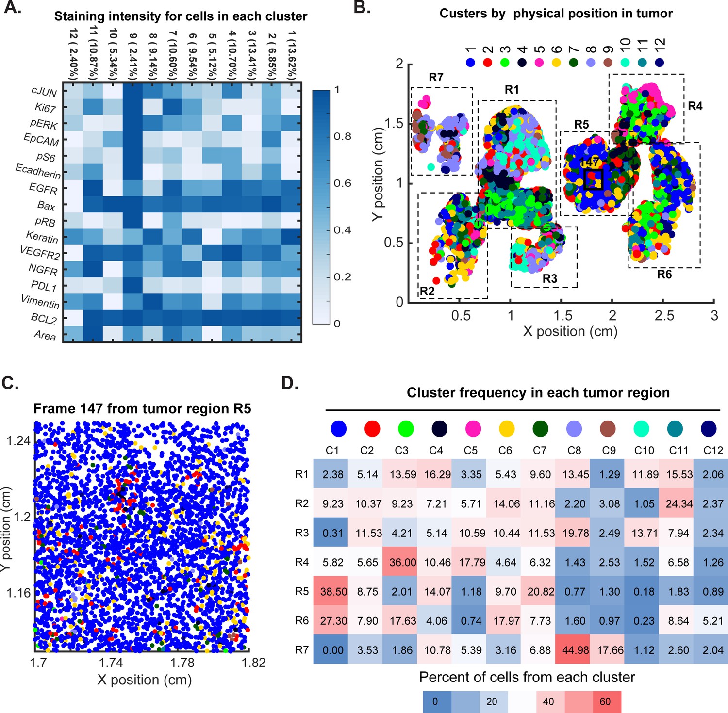
Spatial distribution of molecular phenotypes in a single GBM.
This analysis is directly analogous to the analysis shown in Figure 11, but uses 12 clusters for EMGM analysis rather than 8. (A) Intensity values from the tumor in Figure 10 were clustered using expected-maximization with Gaussian mixtures (EMGM) with k = 12. The number of cells in each cluster is shown as a percentage of all cells in the tumor. (B) EMGM clusters (in color code) mapped back to singles cells and their positions in the tumor. The coordinate system is the same as in Figure 10. The positions of seven macroscopic regions (R1-R7) representing distinct lobes of the tumour are shown. (C) Magnified view of Frame 147 from region R5 with EMGM cluster assignment for each cell in the frame shown as a dot. (D) The proportional representation of EMGM clusters in each tumor region as defined in Panel B.
Tables
Table 1
Microscopes used in this study and their properties.
https://doi.org/10.7554/eLife.31657.009| Instrument | Type | Objective | Field of view | Nominal Resolution* |
|---|---|---|---|---|
| RareCyte Cytefinder | Slide Scanner | 10X/0.3 NA | 1.6 × 1.4 mm | 1.06 µm |
| 20X/0.8NA | 0.8 × 0.7 mm | 0.40 µm | ||
| 40X/0.6 NA | 0.42 × 0.35 mm | 0.53 µm | ||
| GE INCell Analyzer 6000 | Confocal | 60X/0.95 NA | 0.22 × 0.22 mm | 0.21 µm |
| GE OMX Blaze | Structured Illumination Microscope | 60 × 1.42 NA | 0.08 × 0.08 mm | 0.11 µm |
-
*Except in the case of the OMX Blaze, nominal resolution was calculated using the formula (r) = 0.61λ/NA for widefield and (r) = 0.4λ/NA for confocal microscopy with λ = 520 nm. Actual resolution depends on optical properties and thickness of sample, alignment and quality of the optical components in the light path. For structured illumination microscopy, actual resolution depends on accurate matching of immersion oil refractive index with sample in the Cy3 channel and use of an optimal point spread function during reconstruction process. The resolution in other channels will be sub-nominal.
Table 2
List of antibodies tested and validated for t-CyCIF.
https://doi.org/10.7554/eLife.31657.011| Antibody name | Target protein | Performance | Vendor | Catalog no. | Clone | Fluorophore | Research resource Identifier |
|---|---|---|---|---|---|---|---|
| Bax-488 | Bax | * | BioLegend | 633603 | 2D2 | Alexa Fluor 488 | AB_2562171 |
| CD11b-488 | CD11b | * | Abcam | AB204271 | EPR1344 | Alexa Fluor 488 | |
| CD4-488 | CD4 | * | R and D Systems | FAB8165G | Polyclonal | Alexa Fluor 488 | |
| CD8a-488 | CD8 | * | eBioscience | 53-0008-80 | AMC908 | Alexa Fluor 488 | AB_2574412 |
| cJUN-488 | cJUN | * | Abcam | AB193780 | E254 | Alexa Fluor 488 | |
| CK18-488 | Cytokeratin 18 | * | eBioscience | 53-9815-80 | LDK18 | Alexa Fluor 488 | AB_2574480 |
| CK8-FITC | Cytokeratin 8 | * | eBioscience | 11-9938-80 | LP3K | FITC | AB_10548518 |
| CycD1-488 | CycD1 | * | Abcam | AB190194 | EPR2241 | Alexa Fluor 488 | |
| Ecad-488 | E-Cadherin | * | CST | 3199 | 24E10 | Alexa Fluor 488 | AB_10691457 |
| EGFR-488 | EGFR | * | CST | 5616 | D38B1 | Alexa Fluor 488 | AB_10691853 |
| EpCAM-488 | EpCAM | * | CST | 5198 | VU1D9 | Alexa Fluor 488 | AB_10692105 |
| HES1-488 | HES1 | * | Abcam | AB196328 | EPR4226 | Alexa Fluor 488 | |
| Ki67-488 | Ki67 | * | CST | 11882 | D3B5 | Alexa Fluor 488 | AB_2687824 |
| LaminA/C-488 | Lamin A/C | * | CST | 8617 | 4C11 | Alexa Fluor 488 | AB_10997529 |
| LaminB1-488 | Lamin B1 | * | Abcam | AB194106 | EPR8985(B) | Alexa Fluor 488 | |
| mCD3E-FITC | ms_CD3E | * | BioLegend | 100306 | 145–2 C11 | FITC | AB_312671 |
| mCD4-488 | ms_CD4 | * | BioLegend | 100532 | RM4-5 | Alexa Fluor 488 | AB_493373 |
| MET-488 | c-MET | * | CST | 8494 | D1C2 | Alexa Fluor 488 | AB_10999405 |
| mF4/80-488 | ms_F4/80 | * | BioLegend | 123120 | BM8 | Alexa Fluor 488 | AB_893479 |
| MITF-488 | MITF | * | Abcam | AB201675 | D5 | Alexa Fluor 488 | |
| Ncad-488 | N-Cadherin | * | BioLegend | 350809 | 8C11 | Alexa Fluor 488 | AB_11218797 |
| p53-488 | p53 | * | CST | 5429 | 7F5 | Alexa Fluor 488 | AB_10695458 |
| PCNA-488 | PCNA | * | CST | 8580 | PC10 | Alexa Fluor 488 | AB_11178664 |
| PD1-488 | PD1 | * | CST | 15131 | D3W4U | Alexa Fluor 488 | |
| PDI-488 | PDI | * | CST | 5051 | C81H6 | Alexa Fluor 488 | AB_10950503 |
| pERK-488 | pERK(T202/Y204) | * | CST | 4344 | D13.14.4E | Alexa Fluor 488 | AB_10695876 |
| pNDG1-488 | pNDG1(T346) | * | CST | 6992 | D98G11 | Alexa Fluor 488 | AB_10827648 |
| POL2A-488 | POL2A | * | Novus Biologicals | NB200-598AF488 | 4H8 | Alexa Fluor 488 | AB_2167465 |
| pS6(S240/244)−488 | pS6(240/244) | * | CST | 5018 | D68F8 | Alexa Fluor 488 | AB_10695861 |
| S100a-488 | S100alpha | * | Abcam | AB207367 | EPR5251 | Alexa Fluor 488 | |
| SQSTM1-488 | SQSTM1/p62 | * | CST | 8833 | D1D9E3 | Alexa Fluor 488 | |
| STAT3-488 | STAT3 | * | CST | 14047 | B3Z2G | Alexa Fluor 488 | |
| Survivin-488 | Survivin | * | CST | 2810 | 71G4B7 | Alexa Fluor 488 | AB_10691462 |
| Catenin-488 | β-Catenin | * | CST | 2849 | L54E2 | Alexa Fluor 488 | AB_10693296 |
| Actin-555 | Actin | * | CST | 8046 | 13E5 | Alexa Fluor 555 | AB_11179208 |
| CD11c-570 | CD11c | * | eBioscience | 41-9761-80 | 118/A5 | eFluor 570 | AB_2573632 |
| CD3D-555 | CD3D | * | Abcam | AB208514 | EP4426 | Alexa Fluor 555 | |
| CD4-570 | CD4 | * | eBioscience | 41-2444-80 | N1UG0 | eFluor 570 | AB_2573601 |
| CD45-PE | CD45 | * | R and D Systems | FAB1430P-100 | 2D1 | PE | AB_2237898 |
| CK7-555 | Cytokeratin 7 | * | Abcam | AB209601 | EPR17078 | Alexa Fluor 555 | |
| cMYC-555 | cMYC | * | Abcam | AB201780 | Y69 | Alexa Fluor 555 | |
| E2F1-555 | E2F1 | * | Abcam | AB208078 | EPR3818(3) | Alexa Fluor 555 | |
| Ecad-555 | E-Cadherin | * | CST | 4295 | 24E10 | Alexa Fluor 555 | |
| EpCAM-PE | EpCAM | * | BioLegend | 324205 | 9C4 | PE | AB_756079 |
| FOXO1a-555 | FOXO1a | * | Abcam | AB207244 | EP927Y | Alexa Fluor 555 | |
| FOXP3-570 | FOXP3 | * | eBioscience | 41-4777-80 | 236A/E7 | eFluor 570 | AB_2573608 |
| GFAP-570 | GFAP | * | eBioscience | 41-9892-80 | GA5 | eFluor 570 | AB_2573655 |
| HSP90-PE | HSP90b | * | Abcam | AB115641 | Polyclonal | PE | AB_10936222 |
| KAP1-594 | KAP1 | * | BioLegend | 619304 | 20A1 | Alexa Fluor 594 | AB_2563298 |
| Keratin-555 | pan-Keratin | * | CST | 3478 | C11 | Alexa Fluor 555 | AB_10829040 |
| Keratin-570 | pan-Keratin | * | eBioscience | 41-9003-80 | AE1/AE3 | eFluor 570 | AB_11217482 |
| Ki67-570 | Ki67 | * | eBioscience | 41-5699-80 | 20Raj1 | eFluor 570 | AB_11220088 |
| LC3-555 | LC3 | * | CST | 13173 | D3U4C | Alexa Fluor 555 | |
| MAP2-570 | MAP2 | * | eBioscience | 41-9763-80 | AP20 | eFluor 570 | AB_2573634 |
| pAUR-555 | pAUR1/2/3(T288/T2 | * | CST | 13464 | D13A11 | Alexa Fluor 555 | |
| pCHK2-PE | pChk2(T68) | * | CST | 12812 | C13C1 | PE | |
| PDL1-555 | PD-L1/CD274 | * | Abcam | AB213358 | 28–8 | Alexa Fluor 555 | |
| pH3-555 | pH3(S10) | * | CST | 3475 | D2C8 | Alexa Fluor 555 | AB_10694639 |
| pRB-555 | pRB(S807/811) | * | CST | 8957 | D20B12 | Alexa Fluor 555 | |
| pS6(235/236)–555 | pS6(235/236) | * | CST | 3985 | D57.2.2E | Alexa Fluor 555 | AB_10693792 |
| pSRC-PE | pSRC(Y418) | * | eBioscience | 12-9034-41 | SC1T2M3 | PE | AB_2572680 |
| S6-555 | S6 | * | CST | 6989 | 54D2 | Alexa Fluor 555 | AB_10828226 |
| SQSTM1-555 | SQSTM1/p62 | * | Abcam | AB203430 | EPR4844 | Alexa Fluor 555 | |
| VEGFR2-555 | VEGFR2 | * | CST | 12872 | D5B1 | Alexa Fluor 555 | |
| VEGFR2-PE | VEGFR2 | * | CST | 12634 | D5B1 | PE | |
| Vimentin-555 | Vimentin | * | CST | 9855 | D21H3 | Alexa Fluor 555 | AB_10859896 |
| Vinculin-570 | Vinculin | * | eBioscience | 41-9777-80 | 7F9 | eFluor 570 | AB_2573646 |
| gH2ax-PE | gH2ax | * | BioLegend | 613412 | 2F3 | PE | AB_2616871 |
| AKT-647 | AKT | * | CST | 5186 | C67E7 | Alexa Fluor 647 | AB_10695877 |
| aSMA-660 | aSMA | * | eBioscience | 50-9760-80 | 1A4 | eFluor 660 | AB_2574361 |
| B220-647 | CD45R/B220 | * | BioLegend | 103226 | RA3-6B2 | Alexa Fluor 647 | AB_389330 |
| Bcl2-647 | Bcl2 | * | BioLegend | 658705 | 100 | Alexa Fluor 647 | AB_2563279 |
| Catenin-647 | Beta-Catenin | * | CST | 4627 | L54E2 | Alexa Fluor 647 | AB_10691326 |
| CD20-660 | CD20 | * | eBioscience | 50-0202-80 | L26 | eFluor 660 | AB_11151691 |
| CD45-647 | CD45 | * | BioLegend | 304020 | HI30 | Alexa Fluor 647 | AB_493034 |
| CD8a-660 | CD8 | * | eBioscience | 50-0008-80 | AMC908 | eFluor 660 | AB_2574148 |
| CK5-647 | Cytokeratin 5 | * | Abcam | AB193895 | EP1601Y | Alexa Fluor 647 | |
| CoIIV-647 | Collagen IV | * | eBioscience | 51-9871-80 | 1042 | Alexa Fluor 647 | AB_10854267 |
| COXIV-647 | COXIV | * | CST | 7561 | 3E11 | Alexa Fluor 647 | AB_10994876 |
| cPARP-647 | cPARP | * | CST | 6987 | D64E10 | Alexa Fluor 647 | AB_10858215 |
| FOXA2-660 | FOXA2 | * | eBioscience | 50-4778-82 | 3C10 | eFluor 660 | AB_2574221 |
| FOXP3-647 | FOXP3 | * | BioLegend | 320113 | 206D | Alexa Fluor 647 | AB_439753 |
| gH2ax-647 | H2ax(S139) | * | CST | 9720 | 20E3 | Alexa Fluor 647 | AB_10692910 |
| gH2ax-647 | H2ax(S139) | * | BioLegend | 613407 | 2F3 | Alexa Fluor 647 | AB_2114994 |
| HES1-647 | HES1 | * | Abcam | AB196577 | EPR4226 | Alexa Fluor 647 | |
| Ki67-647 | Ki67 | * | CST | 12075 | D3B5 | Alexa Fluor 647 | |
| Ki67-647 | Ki67 | * | BioLegend | 350509 | Ki-67 | Alexa Fluor 647 | AB_10900810 |
| mCD45-647 | ms_CD45 | * | BioLegend | 103124 | 30-F11 | Alexa Fluor 647 | AB_493533 |
| mCD4-647 | ms_CD4 | * | BioLegend | 100426 | GK1.5 | Alexa Fluor 647 | AB_493519 |
| mEPCAM-647 | ms_EPCAM | * | BioLegend | 118211 | G8.8 | Alexa Fluor 647 | AB_1134104 |
| MHCI-647 | MHCI/HLAA | * | Abcam | AB199837 | EP1395Y | Alexa Fluor 647 | |
| MHCII-647 | MHCII | * | Abcam | AB201347 | EPR11226 | Alexa Fluor 647 | |
| mLy6C-647 | ms_Ly6C | * | BioLegend | 128009 | HK1.4 | Alexa Fluor 647 | AB_1236551 |
| mTOR-647 | mTOR | * | CST | 5048 | 7C10 | Alexa Fluor 647 | AB_10828101 |
| NFkB-647 | NFkB (p65) | * | Abcam | AB190589 | E379 | Alexa Fluor 647 | |
| NGFR-647 | NGFR/CD271 | * | Abcam | AB195180 | EP1039Y | Alexa Fluor 647 | |
| NUP98-647 | NUP98 | * | CST | 13393 | C39A3 | Alexa Fluor 647 | |
| p21-647 | p21 | * | CST | 8587 | 12D1 | Alexa Fluor 647 | AB_10892861 |
| p27-647 | p27 | * | Abcam | AB194234 | Y236 | Alexa Fluor 647 | |
| pATM-660 | pATM(S1981) | * | eBioscience | 50-9046-41 | 10H11.E12 | eFluor 660 | AB_2574312 |
| PAX8-647 | PAX8 | * | Abcam | AB215953 | EPR18715 | Alexa Fluor 647 | |
| PDL1-647 | PD-L1/CD274 | * | CST | 15005 | E1L3N | Alexa Fluor 647 | |
| pMK2-647 | pMK2(T334) | * | CST | 4320 | 27B7 | Alexa Fluor 647 | AB_10695401 |
| pmTOR-660 | pmTOR(S2448) | * | eBioscience | 50-9718-41 | MRRBY | eFluor 660 | AB_2574351 |
| pS6_235–647 | pS6(S235/S236) | * | CST | 4851 | D57.2.2E | Alexa Fluor 647 | AB_10695457 |
| pSTAT3-647 | pSTAT3(Y705) | * | CST | 4324 | D3A7 | Alexa Fluor 647 | AB_10694637 |
| pTyr-647 | p-Tyrosine | * | CST | 9415 | p-Tyr-100 | Alexa Fluor 647 | AB_10693160 |
| S100A4-647 | S100A4 | * | Abcam | AB196168 | EPR2761(2) | Alexa Fluor 647 | |
| Survivin-647 | Survivin | * | CST | 2866 | 71G4B7 | Alexa Fluor 647 | AB_10698609 |
| TUBB3-647 | TUBB3 | * | BioLegend | 657405 | AA10 | Alexa Fluor 647 | AB_2563609 |
| Tubulin-647 | beta-Tubulin | * | CST | 3624 | 9F3 | Alexa Fluor 647 | AB_10694204 |
| Vimentin-647 | Vimentin | * | BioLegend | 677807 | O91D3 | Alexa Fluor 647 | AB_2616801 |
| anti-14-3-3 | 14-3-3 | * | Santa Cruz | SC-629-G | Polyclonal | N/D | AB_630820 |
| anti-53BP1 | 53BP1 | * | Bethyl | A303-906A | Polyclonal | N/D | AB_2620256 |
| anti-5HMC | 5HMC | * | Active Motif | 39769 | Polyclonal | N/D | AB_10013602 |
| anti-CD11b | CD11b | * | Abcam | AB133357 | EPR1344 | N/D | AB_2650514 |
| anti-CD2 | CD2 | * | Abcam | AB37212 | Polyclonal | N/D | AB_726228 |
| anti-CD20 | CD20 | * | Dako | M0755 | L26 | N/D | AB_2282030 |
| anti-CD3 | CD3 | * | Dako | A0452 | Polyclonal | N/D | AB_2335677 |
| anti-CD4 | CD4 | * | Dako | M7310 | 4B12 | N/D | |
| anti-CD45RO | CD45RO | * | Dako | M0742 | UCHL1 | N/D | AB_2237910 |
| anti-CD8 | CD8 | * | Dako | M7103 | C8/144B | N/D | AB_2075537 |
| anti-CycA2 | CycA2 | * | Abcam | AB38 | E23.1 | N/D | AB_304084 |
| anti-ET1 | ET-1 | * | Abcam | AB2786 | TR.ET.48.5 | N/D | AB_303299 |
| anti-FAP | FAP | * | eBioscience | BMS168 | F11-24 | N/D | AB_10597443 |
| anti-FOXP3 | FOXP3 | * | BioLegend | 320102 | 206D | N/D | AB_430881 |
| anti-LAMP2 | LAMP2 | * | Abcam | AB25631 | H4B4 | N/D | AB_470709 |
| anti-MCM6 | MCM6 | * | Santa Cruz | SC-9843 | Polyclonal | N/D | AB_2142543 |
| anti-PAX8 | PAX8 | * | Abcam | AB191870 | EPR18715 | N/D | |
| anti-PD1 | PD1 | * | CST | 86163 | D4W2J | N/D | |
| anti-pEGFR | pEGFR(Y1068) | * | CST | 3777 | D7A5 | N/D | AB_2096270 |
| anti-pERK | pERK(T202/Y204) | * | CST | 4370 | D13.14.4E | N/D | AB_2315112 |
| anti-pRB | pRB(S807/811) | * | Santa Cruz | SC-16670 | Polyclonal | N/D | AB_655250 |
| anti-pRPA32 | pRPA32 (S4/S8) | * | Bethyl | IHC-00422 | Polyclonal | N/D | AB_1659840 |
| anti-pSTAT3 | pSTAT3 | ** | CST | 9145 | D3A7 | N/D | AB_2491009 |
| anti-pTyr | pTyr | * | CST | 9411 | p-Tyr-100 | N/D | AB_331228 |
| anti-RPA32 | RPA32 | * | Bethyl | IHC-00417 | Polyclonal | N/D | AB_1659838 |
| anti-TPCN2 | TPCN2 | * | NOVUSBIO | NBP1-86923 | Polyclonal | N/D | AB_11021735 |
| anti-VEGFR1 | VEGFR1/FLT1 | * | Santa Cruz | SC-31173 | Polyclonal | N/D | AB_2106885 |
| Abeta-488 | Beta-Amyloid (1-16) | † | BioLegend | 803013 | 6E10 | Alexa Fluor 488 | AB_2564765 |
| BRAF-FITC | B-RAF | † | Abcam | ab175637 | K21-F | FITC | |
| BrdU-488 | BrdU | † | BioLegend | 364105 | 3D4 | Alexa Fluor 488 | AB_2564499 |
| cCasp3-488 | cCasp3 | † | R and D Systems | IC835G-025 | 269518 | Alexa Fluor 488 | |
| CD11b-488 | CD11b | † | BioLegend | 101219 | M1/70 | Alexa Fluor 488 | AB_493545 |
| CD123-488 | CD123 | † | BioLegend | 306035 | 6H6 | Alexa Fluor 488 | AB_2629569 |
| CD49b-FITC | CD49b | † | BioLegend | 359305 | P1E6-C5 | FITC | AB_2562530 |
| CD69-FITC | CD69 | † | BioLegend | 310904 | FN50 | FITC | AB_314839 |
| CD71-FITC | CD71 | † | BioLegend | 334103 | CY1G4 | FITC | AB_1236432 |
| CD80-FITC | CD80 | † | R and D Systems | FAB140F | 37711 | FITC | AB_357027 |
| CD8a-488 | CD8a | † | eBioscience | 53-0086-41 | OKT8 | Alexa Fluor 488 | AB_10547060 |
| CDC2-FITC | CDC2/p34 | † | Santa Cruz | SC-54 FITC | 17 | FITC | AB_627224 |
| CycB1-FITC | CycB1 | † | Santa Cruz | SC-752 FITC | Polyclonal | FITC | AB_2072134 |
| FN-488 | Fibronection | † | Abcam | AB198933 | F1 | Alexa Fluor 488 | |
| IFNG-488 | Interferron-Gamma | † | BioLegend | 502517 | 4S.B3 | Alexa Fluor 488 | AB_493030 |
| IL1-FITC | IL1 | † | BioLegend | 511705 | H1b-98 | FITC | AB_1236434 |
| IL6-FITC | IL6 | † | BioLegend | 501103 | MQ2-13A5 | FITC | AB_315151 |
| mCD31-FITC | ms_CD31 | † | eBioscience | 11-0311-82 | 390 | FITC | AB_465012 |
| mCD8a-488 | ms_CD8a | † | BioLegend | 100726 | 53–6.7 | Alexa Fluor 488 | AB_493423 |
| Nestin-488 | Nestin | † | eBioscience | 53-9843-80 | 10C2 | Alexa Fluor 488 | AB_1834347 |
| NeuN-488 | NeuN | † | Millipore | MAB377X | A60 | Alexa Fluor 488 | AB_2149209 |
| PR-488 | PR/PGR | † | Abcam | AB199224 | YR85 | Alexa Fluor 488 | |
| Snail1-488 | Snail1 | † | eBioscience | 53-9859-80 | 20C8 | Alexa Fluor 488 | AB_2574482 |
| TGFB-FITC | TGFB1 | † | BioLegend | 349605 | TW4-2F8 | FITC | AB_10679043 |
| TNFa-488 | TNFa | † | BioLegend | 502917 | MAb11 | Alexa Fluor 488 | AB_493122 |
| AR-555 | AR | † | CST | 8956 | D6F11 | Alexa Fluor 555 | AB_11129223 |
| CD11a-PE | CD11a | † | BioLegend | 301207 | HI111 | PE | AB_314145 |
| CD11b-555 | CD11b | † | Abcam | AB206616 | EPR1344 | Alexa Fluor 555 | |
| CD131-PE | CD131 | † | BD | 559920 | JORO50 | PE | AB_397374 |
| CD14-PE | CD14 | † | eBioscience | 12–0149 | 61D3 | PE | AB_10597598 |
| CD1a-PE | CD1a | † | BioLegend | 300105 | HI149 | PE | AB_314019 |
| CD1c-PE | CD1c | † | BioLegend | 331505 | L161 | PE | AB_1089000 |
| CD20-PE | CD20 | † | BioLegend | 302305 | 2H7 | PE | AB_314253 |
| CD23-PE | CD23 | † | eBioscience | 12-0232-81 | B3B4 | PE | AB_465592 |
| CD31-PE | CD31 | † | eBioscience | 12-0319-41 | WM-59 | PE | AB_10670623 |
| CD31-PE | CD31 | † | R and D Systems | FAB3567P-025 | 9G11 | PE | AB_2279388 |
| CD34-PE | CD34 | † | Abcam | AB30377 | QBEND/10 | PE | AB_726407 |
| CD45R-e570 | CD45R/B220 | † | eBioscience | 41-0452-80 | RA3-6B2 | eFluor 570 | AB_2573598 |
| CD71-PE | CD71 | † | eBioscience | 12-0711-81 | R17217 | PE | AB_465739 |
| CD86-PE | CD86 | † | BioLegend | 305405 | IT2.2 | PE | AB_314525 |
| CK19-570 | Cytokeratin 19 | † | eBioscience | 41-9898-80 | BA17 | eFluor 570 | AB_11218678 |
| HER2-570 | HER2 | † | eBioscience | 41-9757-80 | MJD2 | eFluor 570 | AB_2573628 |
| IL3-PE | IL3 | † | BD | 554383 | MP2-8F8 | PE | AB_395358 |
| NFATc1-PE | NFATc1 | † | BioLegend | 649605 | 7A6 | PE | AB_2562546 |
| PDL1-PE | PD-L1/CD274 | † | BioLegend | 329705 | 29E.2A3 | PE | AB_940366 |
| pMAPK (T202/Y204) | pERK1/2(T202/Y20 | † | CST | 14095 | 197G2 | PE | |
| pMAPK (Y204/Y187) | pERK1/2(Y204/Y18 | † | CST | 75165 | D1H6G | PE | |
| pSTAT1-PE | pSTAT1(Y705) | † | BioLegend | 686403 | A15158B | PE | AB_2616938 |
| ABCC1-647 | ABCC1 | † | BioLegend | 370203 | QCRL-2 | Alexa Fluor 647 | AB_2566664 |
| AnnexinV-674 | N/D | † | BioLegend | 640911 | NA | Alexa Fluor 647 | AB_2561293 |
| CD103-647 | CD103 | † | BioLegend | 350209 | Ber-ACT8 | Alexa Fluor 647 | AB_10640870 |
| CD25-647 | CD25 | † | BioLegend | 302617 | BC96 | Alexa Fluor 647 | AB_493046 |
| CD31-APC | CD31 | † | eBioscience | 17-0319-41 | WM-59 | APC | AB_10853188 |
| CD68-APC | CD68 | † | BioLegend | 333809 | Y1/82A | APC | AB_10567107 |
| CD8a-647 | CD8a | † | BioLegend | 344725 | SK1 | Alexa Fluor 647 | AB_2563451 |
| CD8a-647 | CD8a | † | R and D Systems | FAB1509R-025 | 37006 | Alexa Fluor 647 | |
| CycE-660 | CycE | † | eBioscience | 50-9714-80 | HE12 | eFluor 660 | AB_2574350 |
| HIF1-647 | HIF1 | † | BioLegend | 359705 | 546–16 | Alexa Fluor 647 | AB_2563331 |
| HP1-647 | HP1 | † | Abcam | AB198391 | EPR5777 | Alexa Fluor 647 | |
| mCD123-APC | ms_CD123 | † | eBioscience | 17-1231-81 | 5B11 | APC | AB_891363 |
| NGFR-647 | NGFR/CD271 | † | BD | 560326 | C40-1457 | Alexa Fluor 647 | AB_1645403 |
| pBTK-660 | pBTK(Y551/Y511) | † | eBioscience | 50-9015-80 | M4G3LN | eFluor 660 | AB_2574306 |
| PD1-647 | PD1 | † | Abcam | AB201825 | EPR4877 (2) | Alexa Fluor 647 | |
| PR-660 | PR/PGR | † | eBioscience | 50-9764-80 | KMC912 | eFluor 660 | AB_2574363 |
| RUNX3-660 | RUNX3 | † | eBioscience | 50-9817-80 | R3-5G4 | eFluor 660 | AB_2574383 |
| SOX2-647 | SOX2 | † | Abcam | AB192075 | Polyclonal | Alexa Fluor 647 | |
| anti-53BP1 | 53BP1 | † | Millipore | MAB3802 | BP13 | N/D | AB_2206767 |
| anti-Axl | Axl | † | R and D | AF154 | Polyclonal | N/D | AB_354852 |
| anti-CD11b | CD11b | † | Abcam | AB52478 | EP1345Y | N/D | AB_868788 |
| anti-CD8a | CD8 | † | eBioscience | 14-0085-80 | C8/144B | N/D | AB_11151339 |
| anti-CEP170 | CEP170 | † | Abcam | AB72505 | Polyclonal | N/D | AB_1268101 |
| anti-cMYC | cMYC | † | BioLegend | 626801 | 9E10 | N/D | AB_2235686 |
| anti-CPS1 | CPS1 | † | Abcam | AB129076 | EPR7493-3 | N/D | AB_11156290 |
| anti-E2F1 | E2F1 | † | ThermoFisher | MS-879-P1 | KH95 | N/D | AB_143934 |
| anti-eEF2K | eEF2K | † | Santa Cruz | SC-21642 | K-19 | N/D | AB_640043 |
| anti-Emil1 | Emil1 | † | Abcam | AB212397 | EMIL/1176 | N/D | |
| anti-FKHRL1 | FKHRL1 | † | Santa Cruz | SC-9812 | Polyclonal | N/D | AB_640608 |
| anti-FLAG | FLAG | † | Sigma | F1804 | M2 | N/D | AB_262044 |
| anti-GranB | Granzyme_B | † | Dako | M7235 | M7235 | N/D | AB_2114697 |
| anti-HMB45 | HMB45 | † | Abcam | AB732 | HMB45 + M2- 7C10 + M2- 9E3 | N/D | AB_305844 |
| anti-HSP90b | HSP90b | † | Santa Cruz | SC-1057 | D-19 | N/D | AB_2121392 |
| anti-IL2Ra | IL2Ra | † | Abcam | AB128955 | EPR6452 | N/D | AB_11141054 |
| anti-LAMP2 | LAMP2 | † | R and D | AF6228 | Polyclonal | N/D | AB_10971818 |
| anti-MITF | MITF | † | Abcam | AB12039 | C5 | N/D | AB_298801 |
| anti-Ncad | N-Cadherin | † | Abcam | AB18203 | Polyclonal | N/D | AB_444317 |
| anti-NCAM | NCAM | † | Abcam | AB6123 | ERIC-1 | N/D | AB_2149537 |
| anti-NF1 | NF1 | † | Abcam | AB178323 | McNFn27b | N/D | |
| anti-pCTD | Pol II CTD(S2) | † | Active Motif | 61083 | 3E10 | N/D | AB_2687450 |
| anti-PD1 | PD1 | † | CST | 43248 | EH33 | N/D | |
| anti-pTuberin | pTuberin(S664) | † | Abcam | AB133465 | EPR8202 | N/D | AB_11157389 |
| anti-S100 | S100 | † | Dako | Z0311 | Polyclonal | N/D | AB_10013383 |
| anti-SIRT3 | SIRT3 | † | CST | 2627 | C73E3 | N/D | AB_2188622 |
| anti-TIA1 | TIA1 | † | Santa Cruz | SC-1751 | Polyclonal | N/D | AB_2201433 |
| anti-TLR3 | TLR3 | † | Santa Cruz | SC-8691 | Polyclonal | N/D | AB_2240700 |
| anti-TNFa | TNFa | † | Abcam | AB11564 | MP6-XT3 | N/D | AB_298170 |
| anti-TPCN2 | TPCN2 | † | Abcam | AB119915 | Polyclonal | N/D | AB_10903692 |
| CD11a-FITC | CD11a | ‡ | eBioscience | 11-0119-41 | HI111 | FITC | AB_10597888 |
| CD20-FITC | CD20 | ‡ | BioLegend | 302303 | 2H7 | FITC | AB_314251 |
| CD2-FITC | CD2 | ‡ | BioLegend | 300206 | RPA-2.10 | FITC | AB_314030 |
| CD45RO-488 | CD45RO | ‡ | BioLegend | 304212 | UCHL1 | Alexa Fluor 488 | AB_528823 |
| CD8a-488 | CD8 | ‡ | BioLegend | 301024 | RPA-T8 | Alexa Fluor 488 | AB_2561282 |
| cJUN-FITC | cJUN | ‡ | Santa Cruz | SC-1694 FITC | Polyclonal | FITC | AB_631263 |
| CXCR5-FITC | CXCR5 | ‡ | BioLegend | 356913 | J252D4 | FITC | AB_2561895 |
| Ecad-FITC | Ecad | ‡ | BioLegend | 324103 | 67A4 | FITC | AB_756065 |
| FOXP3-488 | FOXP3 | ‡ | BioLegend | 320011 | 150D | Alexa Fluor 488 | AB_439747 |
| MITF-488 | MITF | ‡ | Novus Biologicals | NB100-56561AF488 | 21D1418 | Alexa Fluor 488 | AB_838580 |
| NCAM-488 | NCAM/CD56 | ‡ | Abcam | AB200333 | EPR2566 | Alexa Fluor 488 | |
| NCAM-FITC | NCAM/CD56 | ‡ | ThermoFisher | 11-0566-41 | TULY56 | FITC | AB_2572458 |
| NGFR-FITC | NGFR/CD271 | ‡ | BioLegend | 345103 | ME20.4 | FITC | AB_1937226 |
| PD1-488 | PD-1 | ‡ | BioLegend | 367407 | NAT105 | Alexa Fluor 488 | AB_2566677 |
| PD1-488 | PD-1 | ‡ | BioLegend | 329935 | EH12.2H7 | Alexa Fluor 488 | AB_2563593 |
| pERK-488 | pERK(T202/Y204) | ‡ | CST | 4374 | E10 | Alexa Fluor 488 | AB_10705598 |
| pERK-488 | pERK(T202/Y204) | ‡ | CST | 4780 | 137F5 | Alexa Fluor 488 | AB_10705598 |
| S100A4-FITC | S100A4 | ‡ | BioLegend | 370007 | NJ-4F3-D1 | FITC | AB_2572073 |
| SOX2-488 | SOX2 | ‡ | BioLegend | 656109 | 14A6A34 | Alexa Fluor 488 | AB_2563956 |
| CD133-PE | CD133 | ‡ | eBioscience | 12-1338-41 | TMP4 | PE | AB_1582258 |
| cMyc-TRITC | cMYC | ‡ | Santa Cruz | SC-40 TRITC | 9E10 | TRITC | AB_627268 |
| cPARP-555 | cPARP | ‡ | CST | 6894 | D64E10 | Alexa Fluor 555 | AB_10830735 |
| CTLA4-PE | CTLA4 | ‡ | BioLegend | 369603 | BNI3 | PE | AB_2566796 |
| GATA3-594 | GATA3 | ‡ | BioLegend | 653816 | 16E10A23 | Alexa Fluor 594 | AB_2563353 |
| GFAP-Cy3 | GFAP | ‡ | Millipore | MAB3402C3 | NA | Cy3 | AB_11213580 |
| Oct4-555 | OCT_4 | ‡ | CST | 4439 | C30A3 | Alexa Fluor 555 | AB_10922586 |
| p21-555 | p21 | ‡ | CST | 8493 | 12D1 | Alexa Fluor 555 | AB_10860074 |
| PD1-PE | PD1 | ‡ | BioLegend | 329905 | EH12.2H7 | PE | AB_940481 |
| PDGFRb-555 | PDGFRb | ‡ | Abcam | AB206874 | Y92 | Alexa Fluor 555 | |
| pSTAT1-555 | pSTAT1 | ‡ | CST | 8183 | 58D6 | Alexa Fluor 555 | AB_10860600 |
| TIM1-PE | TIM1 | ‡ | BioLegend | 353903 | 1D12 | PE | AB_11125165 |
| cCasp3-647 | cCasp3 | ‡ | CST | 9602 | D3E9 | Alexa Fluor 647 | AB_2687881 |
| CD103-APC | CD103 | ‡ | eBioscience | 17-1038-41 | B-Ly7 | APC | AB_10669816 |
| CD3-647 | CD3 | ‡ | BioLegend | 300422 | UCHT1 | Alexa Fluor 647 | AB_493092 |
| CD3-660 | CD3 | ‡ | eBioscience | 50-0037-41 | OKT3 | eFluor 660 | AB_2574150 |
| CD3-APC | CD3 | ‡ | eBioscience | 17-0038-41 | UCHT1 | APC | AB_10804761 |
| CD45RO-APC | CD45RO | ‡ | BioLegend | 304210 | UCHL1 | APC | AB_314426 |
| ER-647 | ER | ‡ | Abcam | AB205851 | EPR4097 | Alexa Fluor 647 | |
| FOXO3a-647 | FOXO3a | ‡ | Abcam | AB196539 | EP1949Y | Alexa Fluor 647 | |
| GZMA-e660 | Granzyme A | ‡ | ThermoFisher | 50-9177-41 | CB9 | eFluor 660 | AB_2574330 |
| GZMB-647 | Granzyme_B | ‡ | BioLegend | 515405 | GB11 | Alexa Fluor 647 | AB_2294995 |
| GZMB-APC | Granzyme_B | ‡ | R and D Systems | IC29051A | 356412 | APC | AB_894691 |
| HER2-647 | HER2 | ‡ | BioLegend | 324412 | 24D2 | Alexa Fluor 647 | AB_2262300 |
| mCD49b-647 | ms_CD49b | ‡ | BioLegend | 103511 | HMα2 | Alexa Fluor 647 | AB_528830 |
| NCAM-647 | NCAM/CD56 | ‡ | BioLegend | 362513 | 5.1H11 | Alexa Fluor 647 | AB_2564086 |
| NCAM-e660 | NCAM/CD56 | ‡ | ThermoFisher | 50-0565-80 | 5tukon56 | eFluor 660 | AB_2574160 |
| pAKT-647 | pAKT | ‡ | CST | 4075 | D9E | Alexa Fluor 647 | AB_10691856 |
| pERK-647 | pERK (T202/Y204) | ‡ | CST | 4375 | E10 | Alexa Fluor 647 | AB_10706777 |
| pERK-647 | pERK (T202/Y204) | ‡ | BioLegend | 369503 | 6B8B69 | Alexa Fluor 647 | AB_2571895 |
| pIKBa-660 | pIKBa | ‡ | eBioscience | 50-9035-41 | RILYB3R | eFluor 660 | AB_2574310 |
| YAP-647 | YAP | ‡ | CST | 38707S | D8H1X | Alexa Fluor 647 | |
| anit-FANCD2 | FANCD2 | ‡ | Bethyl | IHC-00624 | Polyclonal | N/D | AB_10752755 |
| anit-pcJUN | p-cJUN | ‡ | Santa Cruz | SC-822 | KM-1 | N/D | AB_627262 |
| anti-AXL | AXL | ‡ | CST | 8661 | C89E7 | N/D | AB_11217435 |
| anti-CXCR5 | CXCR5 | ‡ | GeneTex | GTX100351 | Polyclonal | N/D | AB_1240668 |
| anti-CXCR5 | CXCR5 | ‡ | R and D | MAB-190-SP | 51505 | N/D | AB_2292654 |
| anti-FOXO3a | FOXO3a | ‡ | CST | 2497 | 75D8 | N/D | AB_836876 |
| anti-GZMB | Granzyme B | ‡ | Abcam | AB4059 | Polyclonal | N/D | AB_304251 |
| anti-PD1 | PD-1 | ‡ | Abcam | AB63477 | Polyclonal | N/D | AB_2159165 |
| anti-PD1 | PD-1 | ‡ | ThermoFisher | 14-9985-81 | J43 | N/D | AB_468663 |
| anti-PD1 | PD-1 | ‡ | R and D | AF1021 | Polyclonal | N/D | AB_354541 |
| anti-RFP | RFP | ‡ | ThermoFisher | R10367 | Polyclonal | N/D | AB_2315269 |
| CD11C-BV570 | CD11C | ‡ | BioLegend | 117331 | N418 | BV570 | AB_10900261 |
| CD45-BV785 | CD45 | ‡ | BioLegend | 304047 | HI30 | BV785 | AB_2563128 |
| LY6G-BV570 | LY6G | ‡ | BioLegend | 127629 | 1A8 | BV570 | AB_10899738 |
-
*Show positive/correct signals in multiple samples/tissues.
†Show positive/correct signals in some but not all samples tested.
-
‡Show no signal or incorrect signals in most samples tested.
Key resources table
| Reagent type (species) or resource | Designation | Source or reference | Identifiers | Additional information |
|---|---|---|---|---|
| Biological sample (human tissue specimen) | TMA:TMA-1207 | Protein Biotechnologies | Cat: TMA-1207 | http://www.proteinbiotechnologies.com/pdf/TMA-1207.pdf |
| Biological sample (human tissue specimen) | TMA:MTU481 | Biomax | Cat: MTU-481 | https://www.biomax.us/tissue-arrays/Multiple_Organ/MTU481 |
| Antibody | Alexa-488 anti-Rabbit antibodies (Fab) | ThermoFisher Scientific | Cat: A-11034 (RRID:AB_2576217) | Dilution 1:2000 |
| Antibody | Alexa-555 anti-Rat antibodies | ThermoFisher Scientific | Cat: A-21434 (RRID:AB_141733) | Dilution 1:2000 |
| Antibody | Alexa-647 anti-Mouse antibodies (Fab) | ThermoFisher Scientific | Cat: A-21236 (RRID:AB_141725) | Dilution 1:2000 |
| Chemical compound, drug | Hoechst 33342 | ThermoFisher Scientific | Cat: H3570 | https://www.thermofisher.com/order/catalog/product/H3570 |
| Software, algorithm | ImageJ | PMID:22930834 | RRID: SCR_003070 | https://imagej.nih.gov/ij/ |
| Software, algorithm | Matlab | MathWorks, Inc. | RRID:SCR_001622 | |
| Software, algorithm | Ashlar | Laboratory of Systems Pharmacology, Harvard Medical School | RRID:SCR_016266 | https://github.com/sorgerlab/ashlar (copy archived at https://github.com/elifesciences-publications/ashlar) |
| Software, algorithm | BaSiC | Helmholtz Zentrum München | RRID: SCR_016371 | https://www.nature.com/articles/ncomms14836 |
| Other | www.cycif.org | Laboratory of Systems Pharmacology, Harvard Medical School | RRID:SCR_016267 | Online resource for cyclic immunofluorescence |
| Other | lincs.hms.harvard.edu | HMS LINCS Center | RRID:SCR_016370 | Additional data/image resource for t-CyCIF |
Table 3
Breakdown of individual steps performed for dewaxing and antigen retrieval on a Leica BOND.
https://doi.org/10.7554/eLife.31657.041| Step | Reagent | Supplier | Incubation (min) | Temp. (°C) |
|---|---|---|---|---|
| 1 | *No Reagent | N/D | 30 | 60 |
| 2 | BOND Dewax Solution | Leica | 0 | 60 |
| 3 | BOND Dewax Solution | Leica | 0 | R.T. |
| 4 | BOND Dewax Solution | Leica | 0 | R.T. |
| 5 | 200 proof ethanol | User* | 0 | R.T. |
| 6 | 200 proof ethanol | User* | 0 | R.T. |
| 7 | 200 proof ethanol | User* | 0 | R.T. |
| 8 | Bond Wash Solution | Leica | 0 | R.T. |
| 9 | Bond Wash Solution | Leica | 0 | R.T. |
| 10 | Bond Wash Solution | Leica | 0 | R.T. |
| 11 | Bond ER1 solution | Leica | 0 | 99 |
| 12 | Bond ER1 solution | Leica | 0 | 99 |
| 13 | Bond ER1 solution | Leica | 20 | 99 |
| 14 | Bond ER1 solution | Leica | 0 | R.T. |
| 15 | Bond Wash Solution | Leica | 0 | R.T. |
| 16 | Bond Wash Solution | Leica | 0 | R.T. |
| 17 | Bond Wash Solution | Leica | 0 | R.T. |
| 18 | Bond Wash Solution | Leica | 0 | R.T. |
| 19 | Bond Wash Solution | Leica | 0 | R.T. |
| 20 | IF Block | User* | 30 | R.T. |
| 21 | Antibody Mix | User* | 60 | R.T. |
| 22 | Bond Wash Solution | Leica | 0 | R.T. |
| 23 | Bond Wash Solution | Leica | 0 | R.T. |
| 24 | Bond Wash Solution | Leica | 0 | R.T. |
| 25 | Hoechst Solution | User* | 30 | R.T. |
| 26 | Bond Wash Solution | Leica | 0 | R.T. |
| 27 | Bond Wash Solution | Leica | 0 | R.T. |
| 28 | Bond Wash Solution | Leica | 0 | R.T. |
Additional files
-
Supplementary file 1
List of antibodies used for staining in Figure 3.
- https://doi.org/10.7554/eLife.31657.042
-
Supplementary file 2
- https://doi.org/10.7554/eLife.31657.043
-
Supplementary file 3
List of antibodies used for staining in Figures 7, 8 and 10.
- https://doi.org/10.7554/eLife.31657.044
-
Supplementary file 4
List of antibodies used for staining in Figure 9.
- https://doi.org/10.7554/eLife.31657.045
-
Supplementary file 5
Descriptions of TMA shown in Figure 10.
- https://doi.org/10.7554/eLife.31657.046
-
Supplementary file 6
List of antibodies used for staining in Figures 11 and 12.
- https://doi.org/10.7554/eLife.31657.047
-
Transparent reporting form
- https://doi.org/10.7554/eLife.31657.048
Download links
A two-part list of links to download the article, or parts of the article, in various formats.
Downloads (link to download the article as PDF)
Open citations (links to open the citations from this article in various online reference manager services)
Cite this article (links to download the citations from this article in formats compatible with various reference manager tools)
Highly multiplexed immunofluorescence imaging of human tissues and tumors using t-CyCIF and conventional optical microscopes
eLife 7:e31657.
https://doi.org/10.7554/eLife.31657


