An optimized method for 3D fluorescence co-localization applied to human kinetochore protein architecture
- University of North Carolina at Chapel Hill, United States
Figures
Figure 1
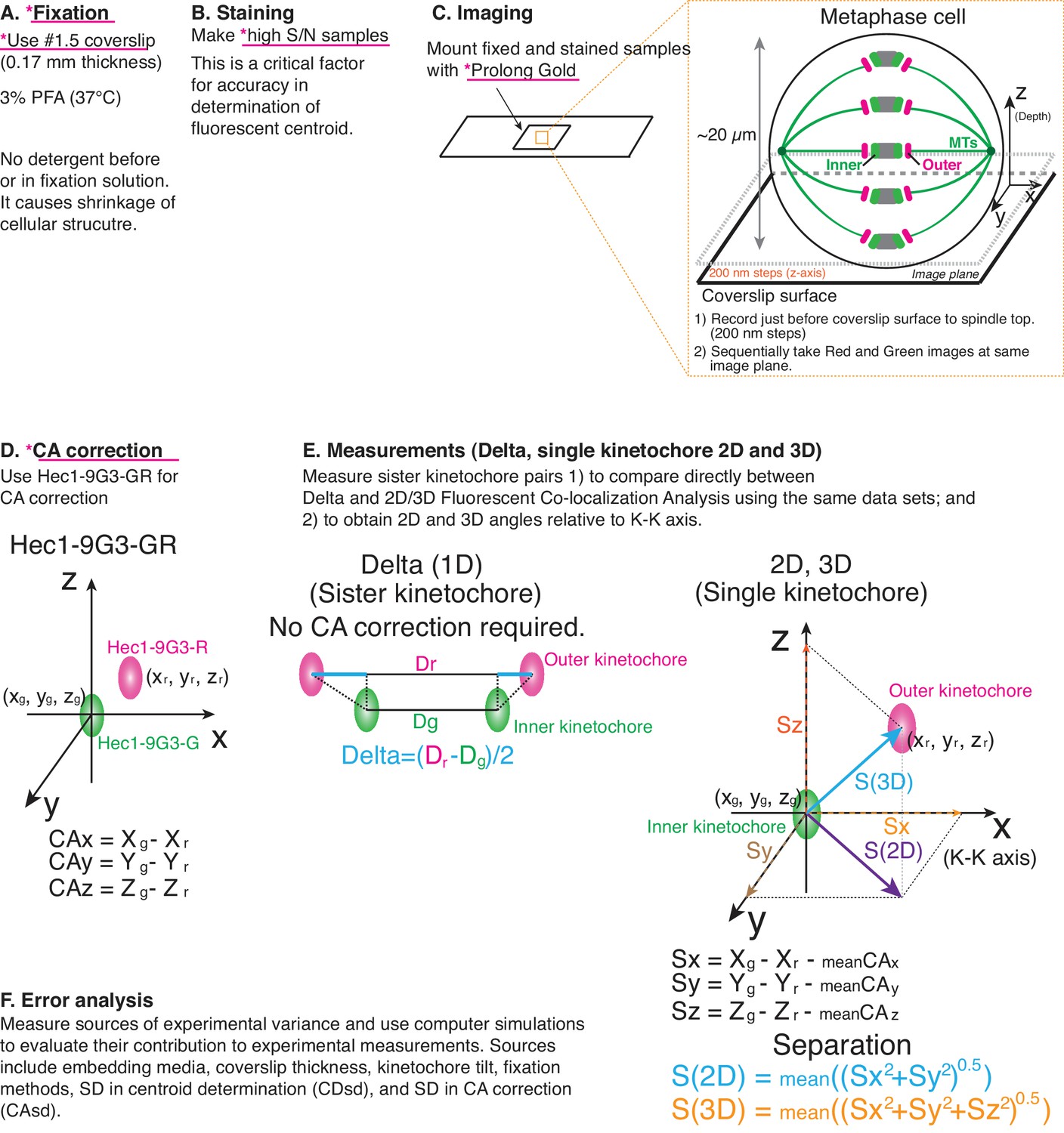
Principle of procedure used in this study.
(A) Fixation: 3% PFA in PHEM buffer without any detergent was used as standard fixation in this study (Details in Text and Methods). (B) Staining: Fixed samples were immunofluorescently labeled with antibodies to enhance S/N. Samples were usually mounted with Prolong Gold. (C) Imaging was performed by spinning disk confocal microscopy (See Materials and methods for details). (D) For CA correction, Hec1-9G3 monoclonal antibody was labeled by green and red tagged secondary antibodies (Hec1-9G3-GR). (E) Measurements: X, Y, Z coordinates of the centroids of green and red kinetochore fluorescence were determined by 3D Gaussian fitting. Details of equations for separation measurements are in Text, Figures, and Methods. (F) Error analysis: computer simulations were used for error analysis of the method. The sources of potential errors in separation measurements were highlighted in pink underline with *.
-
Figure 1—source data 1
Pipeline for obtaining mean 3D separation measurements with nm-scale accuracy.
Critical factors were: (1) prepare bright high signal to noise samples to reduce standard deviation (SD) of centroid determination; (2) use mounting media like ProLong Gold to suppress z-axis spherical aberration; (3) use 0.17 mm thick coverslips for all measurements including CA measurement; (4) align imaging system and image using only a small region within the center of camera to suppress SD of CA; and (5) use warmed PFA fixation without pre-extraction or detergent in fixation solution.
- https://doi.org/10.7554/eLife.32418.003
Figure 2 with 3 supplements
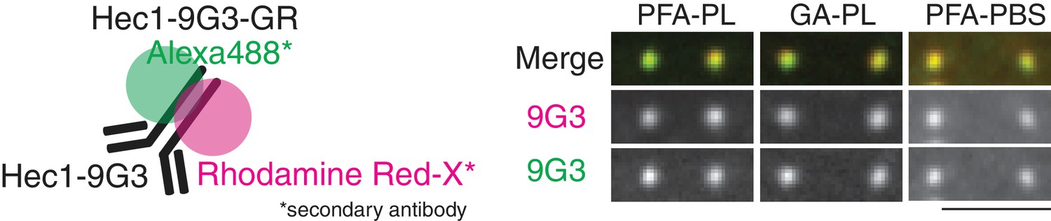
CA (Chromatic aberration) measurements using Hec1-9G3-GR.
Schematic model of Hec1-9G3-GR. Hec1-9G3 antibody was labeled by secondary antibodies with Rhodamine Red-X and Alexa 488 (left). Representative Hec1-9G3-GR images in samples fixed by PFA or GA mounted with Prolong Gold or PBS.
Figure 2—figure supplement 1

CAz is insensitive to depth in samples mounted with Prolong Gold, but not in samples mounted with PBS.
Representative plots of CAz versus depth for experimental conditions in Figure 2A.
Figure 2—figure supplement 2
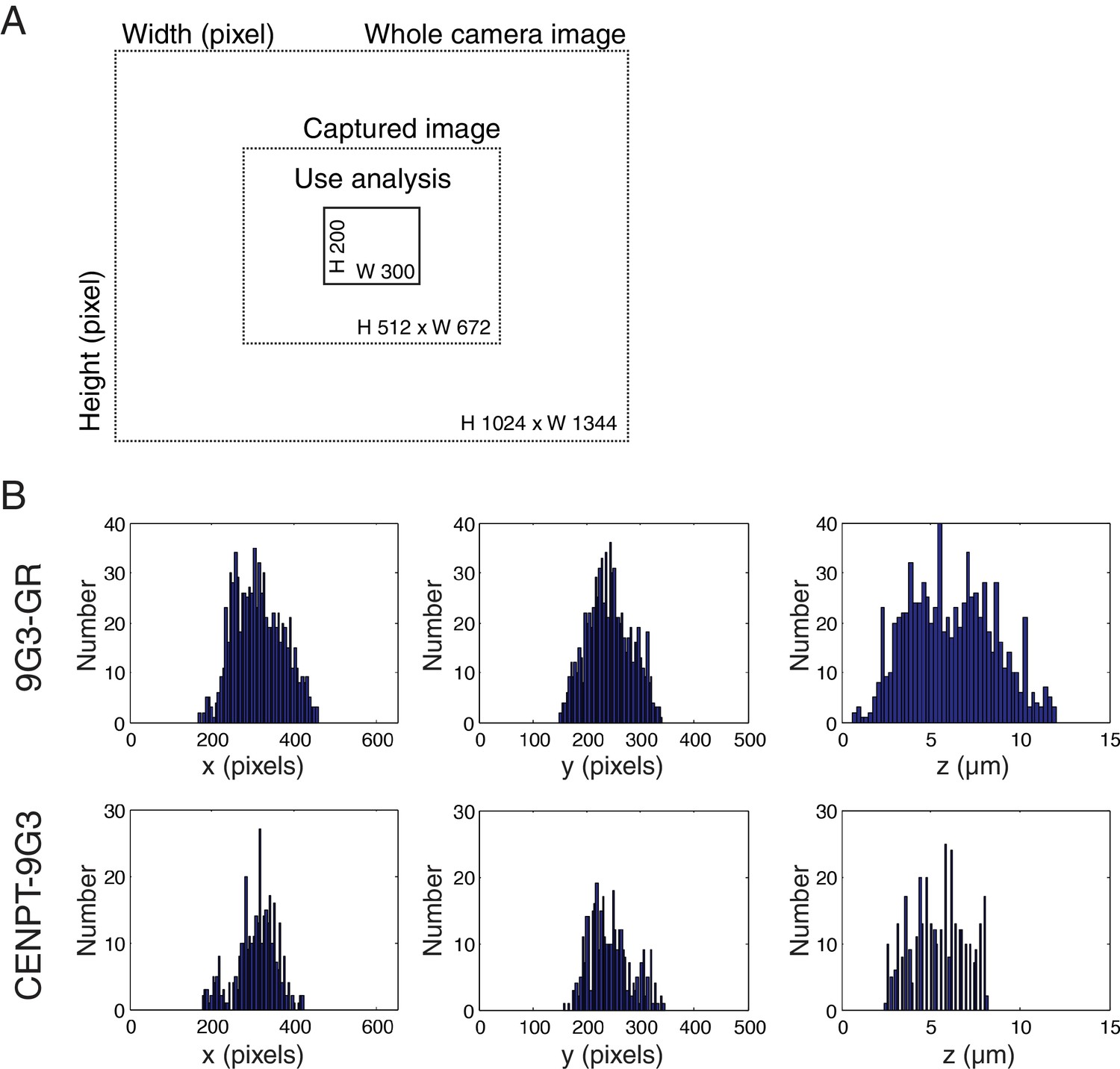
Center of camera image was used for all analysis.
(A) Schematic description of the sizes of the camera detector, captured image, and region used for image analysis. (B) The frequency of kinetochores measured for Hec1(9G3)-GR and CENP-T(M)-Hec1(9G3). They were within the x (300 pixels), y (200 pixels), z (20 µm) imaging region.
Figure 2—figure supplement 3

Measurement of CA of the microscope optics.
Plots of CAx, CAy, and CAz versus x, y, and z for separation between Hec1-9G3-GR in samples fixed with PFA and mounted with Prolong Gold.
Figure 3
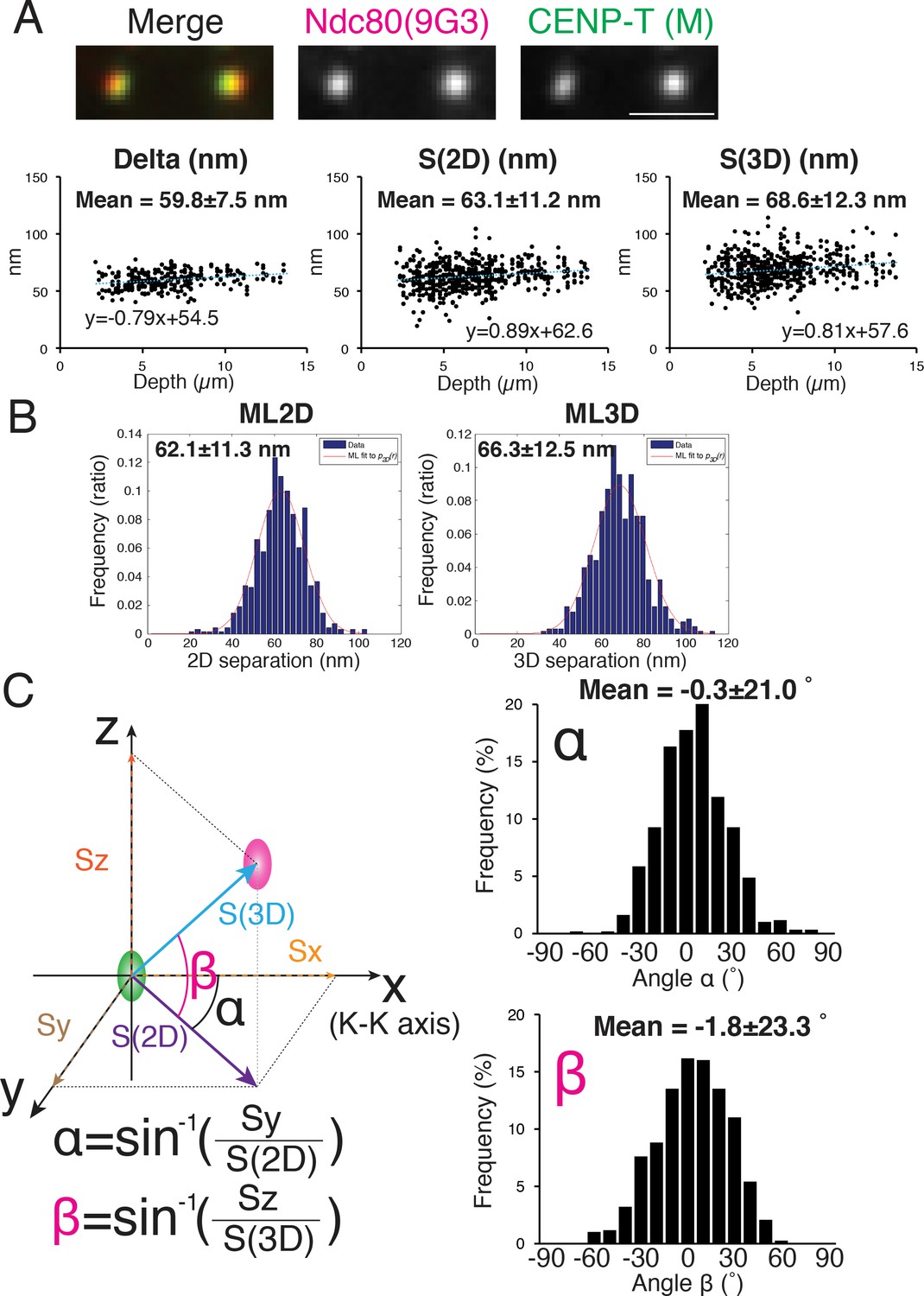
Mean Delta, 2D, and 3D separations between Hec1-9G3 and CENP-T (M).
(A) Representative immunofluorescent (IF) images (top) and plots of Depth verses Delta, S(2D) and S(3D) for the separation between CENP-T(M) and Hec1-9G3 (bottom). (B) Histograms of maximum likelihood fit used to calculate ML2D and ML3D. (C) Orientation of the S(3D) separation vector relative to the sister K-K axis (x-axis in this diagram). Angle α is the rotation of the S(2D) vector component in the x-y plane away from the K-K (x-axis) and angle β is the rotation of the S(3D) vector away from the x-y plane and toward the z-axis (schematic on left). Histograms of α and β values (Right). n > 600 individual kinetochores. All values were mean ±SD. Note, CENP-T(M) is a polyclonal antibody against whole CENP-T protein, and its epitope is not precisely known (Gascoigne et al., 2011).
Figure 4 with 1 supplement
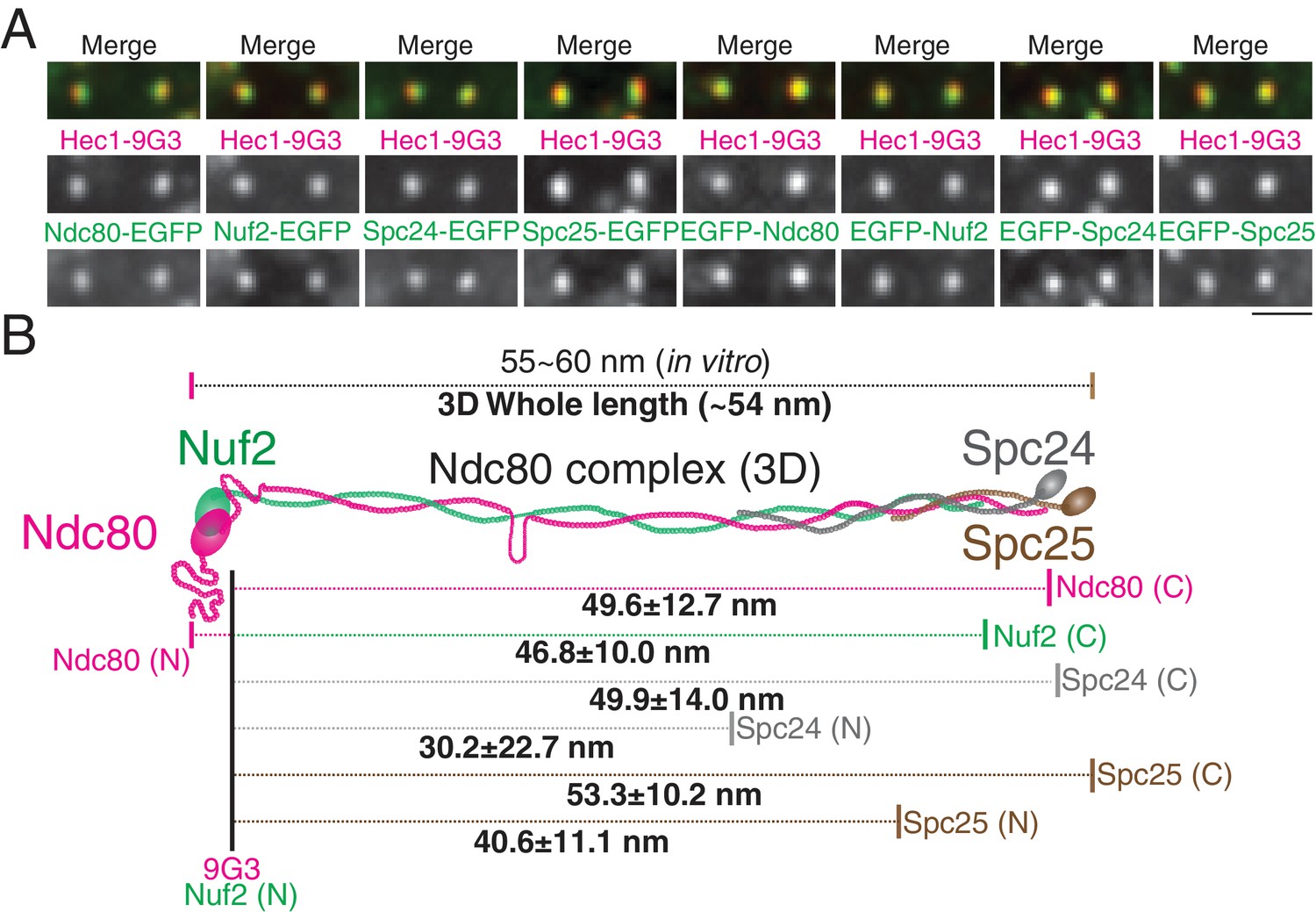
2D/3D co-localization measurements of a structural standard, the extended Ndc80 complex.
(A) Representative immunofluorescent images of Hec1-9G3 and EGFP fused to different protein domains along the Ndc80 complex (See Text and Materials and methods). (B) Schematic summary of the ML3D Ndc80 complex measurements at metaphase. All values were mean ±SD. n > 200 kinetochores for each measurement. Detail values are listed in Figure 4—figure supplement 1.
-
Figure 4—source data 1
The list for Ndc80 complex measurements.
List of mean values of Delta, S(2D), S(3D), ML2D, ML3D between EGFP-Ndc80, Ndc80-EGFP, EGFP-Nuf2, Nuf2-EGFP, EGFP-Spc24, Spc24-EGFP, EGFP-Spc25, or Spc25-EGFP and Hec1-9G3. All values listed are mean ±S.D.
- https://doi.org/10.7554/eLife.32418.012
Figure 4—figure supplement 1
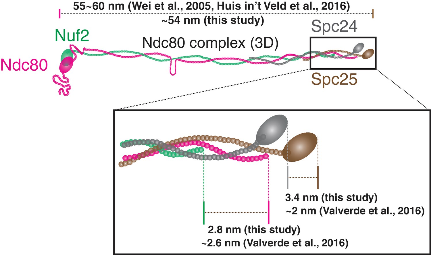
Detailed sub-protein structure of Ndc80 complex.
Schematic picture of the Ndc80 complex with detailed comparison between this study and previous in vitro studies by electron microscopy and crystallography (Wei et al., 2005; Huis In 't Veld et al., 2016; Valverde et al., 2016). Endogenous proteins were depleted by siRNA (See detail in Materials and methods: Suzuki et al., 2015).
Figure 5
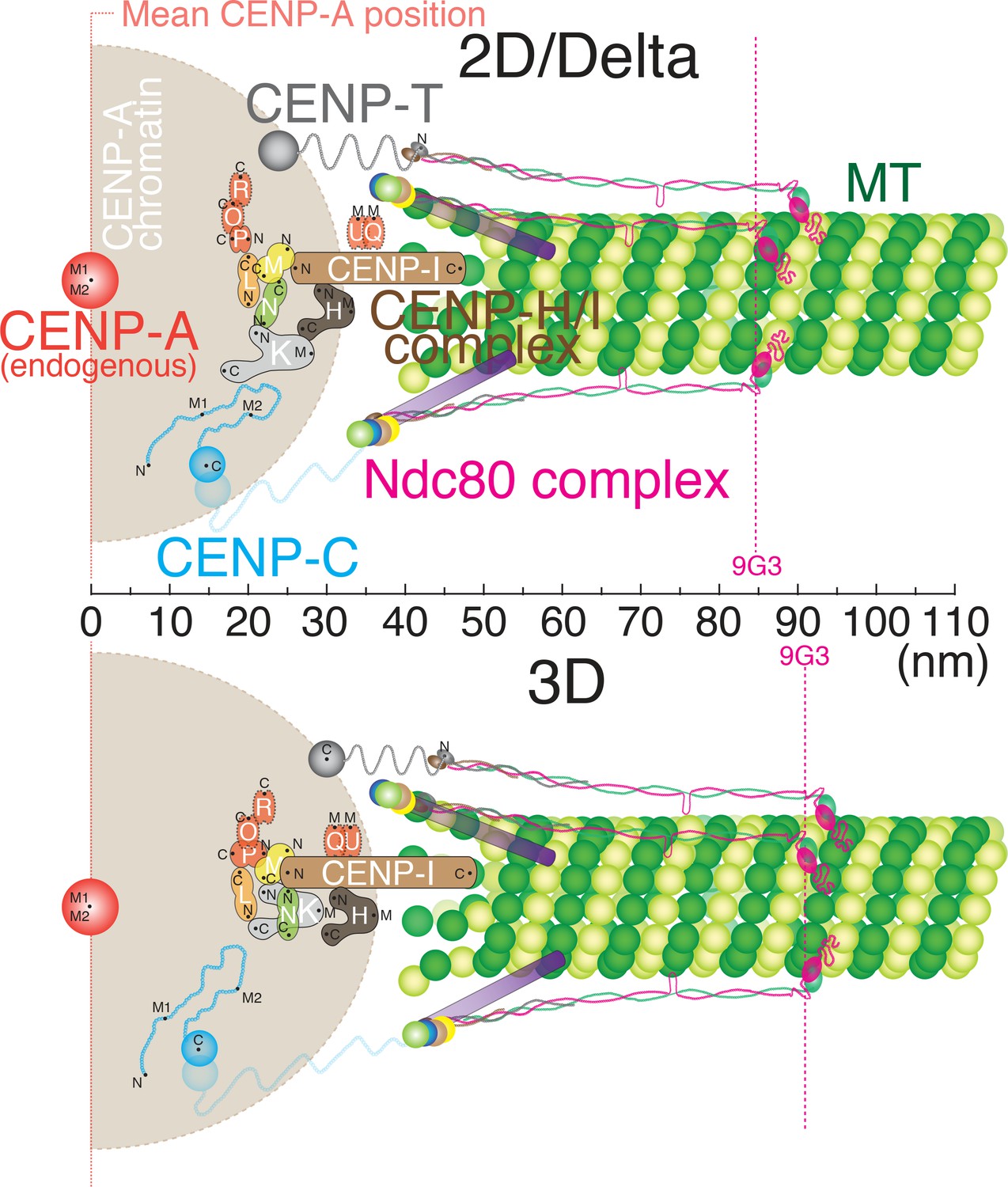
Schematic core-kinetochore drawing measured by 2D/Delta or 3D co-localization method.
Schematic picture of the mean positions of protein labels within the core kinetochore protein architecture measured using ML2D/Delta (top) and ML3D (bottom) methods. N or C are the mean positions of N-terminal or C-terminal EGFP fusions or specific antibodies. M indicates the mean position measured using polyclonal antibodies whose epitope(s) are not precisely known.
-
Figure 5—source data 1
List for core-kinetochore protein measurements.
List of mean values of Delta, S(2D), S(3D), ML2D, ML3D, Z-offset, and zML3D (Z-offset subtracted) for core kinetochore proteins. The differences between ML3D and ML2D (ML3D-ML2D), ML3D and zML3D (ML3D-zML3D) are also listed. All values listed are mean ±S.D.
- https://doi.org/10.7554/eLife.32418.015
-
Figure 5—source data 2
List of primary antibodies.
List of antibodies used in this study with source and references.
- https://doi.org/10.7554/eLife.32418.016
Figure 6 with 2 supplements
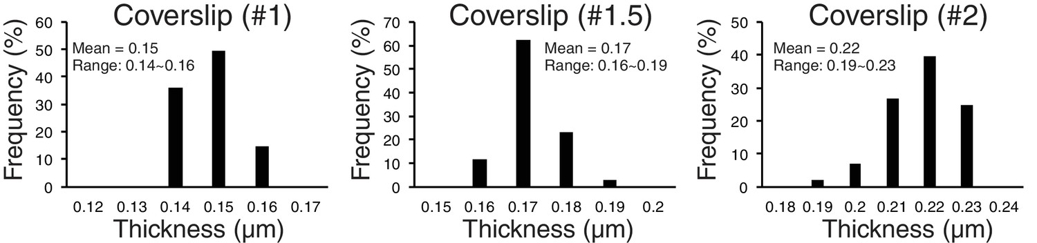
Accuracy of separation measurements depends critically on mean z-axis CA (Z-offset) produced by coverslip thickness variations from standard value.
Measured variability of coverslip thickness within #1, #1.5, and #2 coverslips.
Figure 6—figure supplement 1
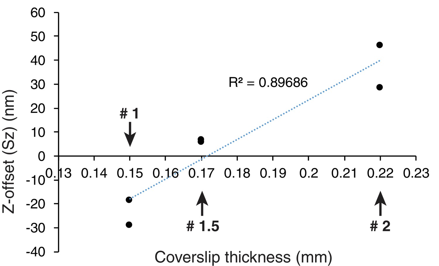
Z-offset changes dependent on coverslip thickness.
The plot of measured Z-offset vs mean coverslip thickness. The mean coverslip thickness was 0.15 mm (#1 coverslip), 0.17 mm (#1.5 coverslip), and 0.22 mm (#2 coverslip).
Figure 6—figure supplement 2
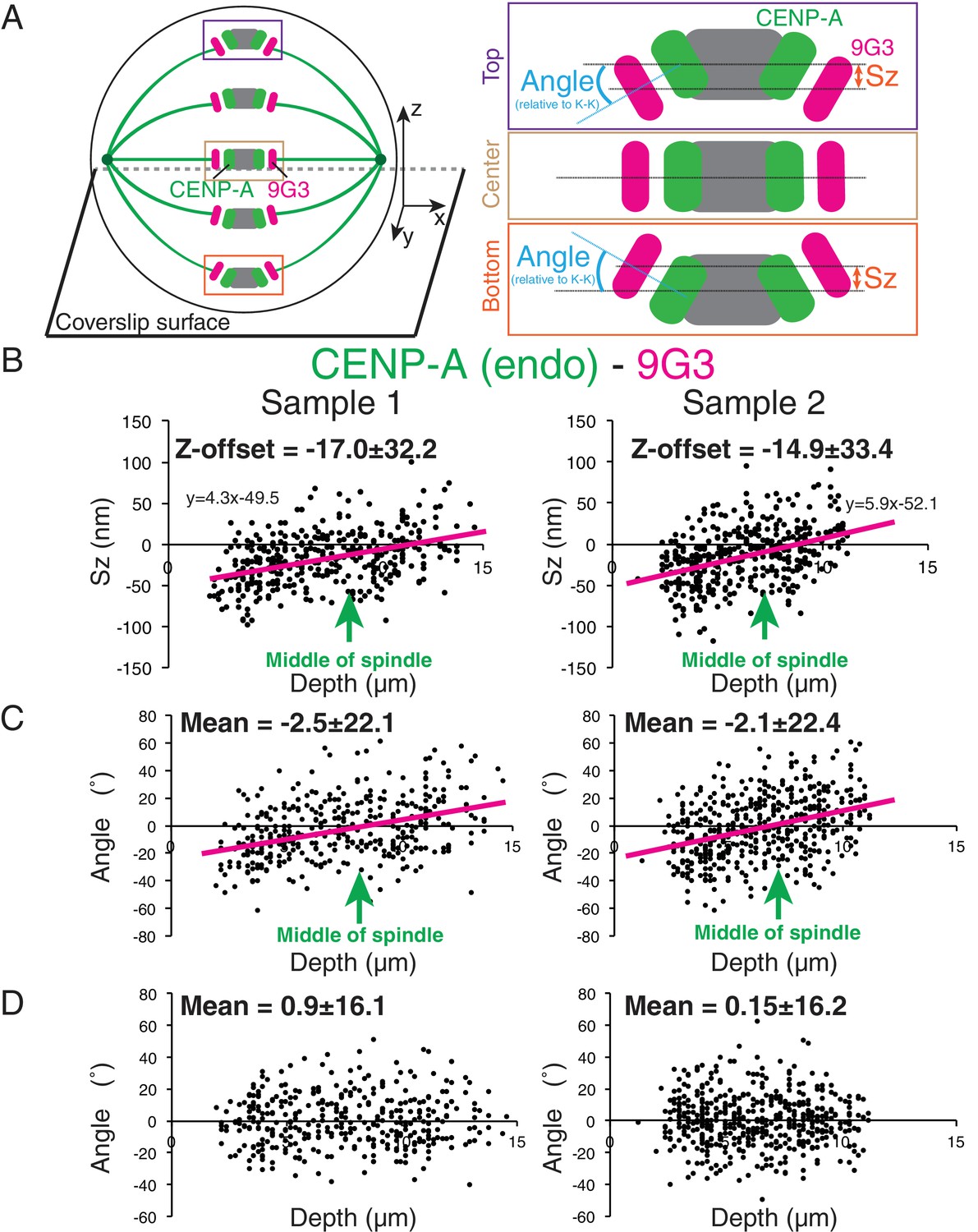
Z-axis offset from kinetochore tilt.
(A) Enlarged view of average kinetochore orientation relative to the K-K axis in metaphase where kinetochores at the bottom half of the spindle are rotated upward in a plus z direction, while kinetochores near the top half of the spindle are rotated downward in a minus z direction to a degree dependent on the kinetochore off-axis position. For a green inner kinetochore label and red outer kinetochore label, rotation makes Sz negative in the bottom half of the spindle and positive in the top half in proportion to the magnitude of label separation. (B) Two examples of Sz versus depth for endogenous CENP-A and Hec1-9G3 separation. (C) Plots of angle β versus depth for the samples in (B). Note, in order to understand kinetochore tilt, angle β for this plot was obtained after subtracting the mean value of Sz at the middle of the spindle from the Sz data for each sample. n > 350 individual kinetochores for each experiment. The arrows in each plot in (B) and (C) indicate the average position of the middle of spindle. (D) Plots of angle α versus depth for the samples in (B).
Figure 7

Comparison of various fixation methods for signal intensity and mean fluorescence co-localization analysis.
(A) Representative immunofluorescent images stained by CENP-T(M) and Hec1-9G3 antibodies using the fixation protocols listed in Table 4. (B) The plots of normalized signal intensity of Hec1-9G3 (left) and CENP-T (right) at kinetochores using the fixation protocols listed in Table 4. The signal intensities were normalized for the mean values of PFA fixation (~20,000 integrated fluorescence counts above local background for Method 1). All values were mean ±SD. n > 200 individual kinetochores for each experiment. **p<0.05 (t-test).
Figure 8
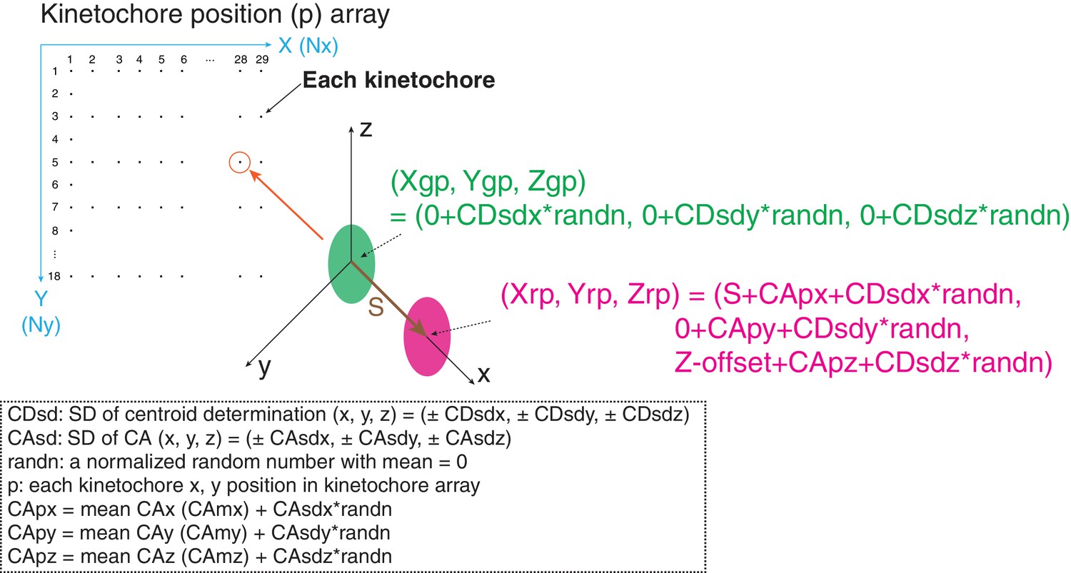
Diagram of simulation model.
We used a 290 × 180 pixel region (x and y) and kinetochores at positions (p) separated by 10 pixels in each direction. All simulated values S(2D), S(3D), angle α, and angle β were averaged from 29 × 18 = 551 kinetochores. The maximum likelihood fit was applied to the raw simulated S(2D) and S(3D) values in the same way as for the experimental analysis in this study.
Figure 9 with 1 supplement
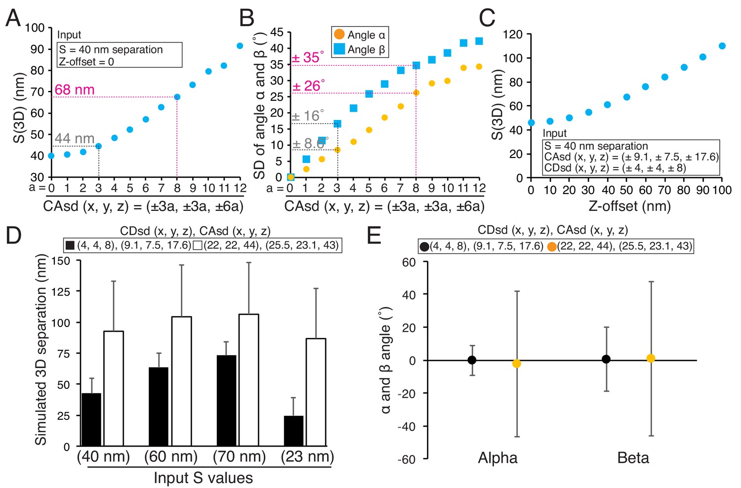
Origins of error in mean separation measurements and comparison of our results to previous reports.
(A) Plots of simulated S(3D) for 40 nm separation with increasing values of CAsd (SD of CA) where the mean CA values were held constant at our measured values of 13.1, 15.8, and 3.5 nm respectively. Grey dashed line is nearly identical to the CAsd for our measurements and the red dashed line is nearly identical to the CAsd for the Smith et al., 2016 measurements. (B) Plots of SD of simulated angle α and β for 60 nm separation using the same condition in (A). (C) Plots of simulated S(3D) for S = 40 nm separation for increasing values of Z-offset and the CAsd reported by Smith et al. (2016). (D) The simulated 3D separation using our SDs (black bars) or in Smith et al. (2016) (white bars). The true separations (S values) are 40, 60, 70, and 23 nm from left to right, which correspond to the mean values from Delta analysis in Table 7. (E) The simulated mean angle α and β with ±SD for the conditions in (E). Note, the input mean angle α and β were zero, and S = 60 nm.
-
Figure 9—source data 1
Estimation of SD for centroid determination (CDsd).
Computer simulations were used with zero CAsd to estimate CDsd (x, y, z) from the SD of Delta measurements (local CA correction) in our study (top) or Smith et al., 2016 (bottom).
- https://doi.org/10.7554/eLife.32418.028
-
Figure 9—source data 2
Estimation of kinetochore-kinetochore variability (Ksd) in our measurements.
The table of experimental or simulated results using fixed S value (60 nm), CDsd ((x, y, z) = (±4, ±4, ±8)), and CAsd ((x, y, z) = (±9.1, ±7.5, ±17.6)) with kinetochore-to-kinetochore variability (Ksd = ±0, ±5, ±10, or ±15 nm).
- https://doi.org/10.7554/eLife.32418.029
Figure 9—figure supplement 1
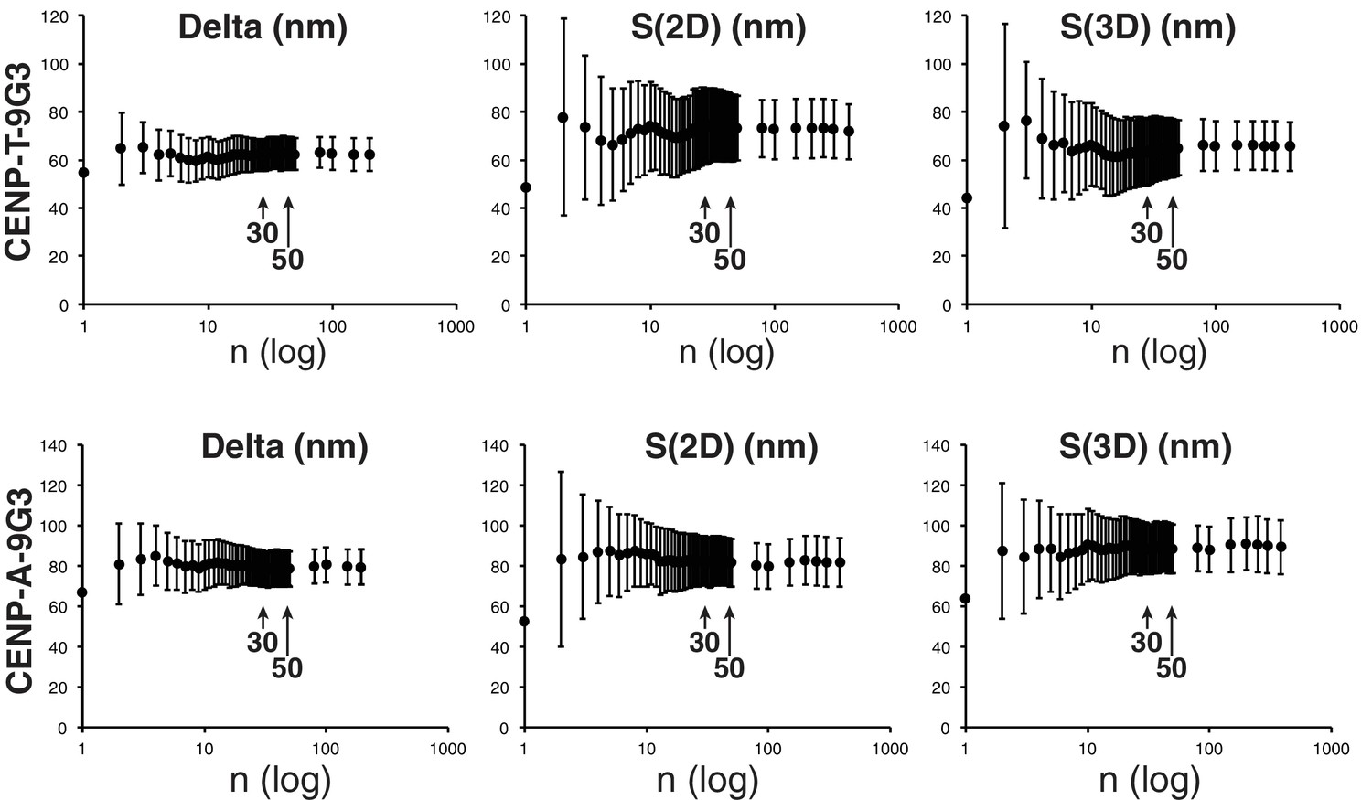
About 10 ~15 kinetochore measurements are sufficient to obtain a mean value close to the mean separation values ± SD from>200 kinetochores.
Plots of mean Delta, S(2D), and S(3D) versus sample number (n, log) for separations between CENP-T and Hec1-9G3, and between endogenous CENP-A and Hec1-9G3.
Tables
Table 1
Mean and SD values of CAx, CAy, CAz for different sample preparations.
https://doi.org/10.7554/eLife.32418.008| Fixation | MM | Green | Red | CAx (nm) | CAy (nm) | CAz (nm) | N | |
|---|---|---|---|---|---|---|---|---|
| Use for correction | PFA | PL | 9G3 | 9G3 | 13.1 ± 9.1 | 15.8 ± 7.5 | 3.5 ± 17.6 | 166 |
| PFA | PL | 9G3 | 9G3 | 14.7 ± 11.4 | 13.2 ± 12.1 | 1.5 ± 17.0 | 256 | |
| PFA | PL | 9G3 | 9G3 | 15.7 ± 12.5 | 15.6 ± 8.2 | −4.8 ± 20.2 | 206 | |
| Use for correction | PFA | PBS | 9G3 | 9G3 | 13.2 ± 10.7 | 18.7 ± 10.4 | −2.7 ± 47.5 | 168 |
| Use for correction | GA | PL | 9G3 | 9G3 | 19.2 ± 10.3 | 16.0 ± 9.0 | −6.8 ± 18.8 | 170 |
Table 2
Comparison of measurements for kinetochores that were part of sister pairs and kinetochores selected at random from a single metaphase cell.
https://doi.org/10.7554/eLife.32418.013| Methods | Green | Red | Delta (nm) | S(2D) (nm) | S(3D) (nm) | ML2D (nm) | ML3D (nm) | n |
|---|---|---|---|---|---|---|---|---|
| Sister pair | Spc25-EGFP | 9G3 | 49.4 ± 4.6 | 51.5 ± 9.6 | 55.2 ± 10.0 | 50.6 ± 9.7 | 53.3 ± 10.2 | 280 (140 pairs) from 6 cells |
| Random | Spc25-EGFP | 9G3 | N.A. | 50.8 ± 6.7 | 55.3 ± 7.7 | 50.3 ± 6.7 | 54.2 ± 7.8 | 120 from single cell |
Table 3
(A) List of Delta, S(2D), S(3D), Z-offset, and zS(3D) (Z-offset subtracted) for the mean separation between CENP-T(M) and Hec1(9G3) in samples with or without large Z-offset.
(B) List of Delta, S(2D), S(3D), Z-offset, and zS(3D) in samples with #1, #1.5, and #2 coverslips. The value zS(3D) was calculated from the S(3D) data after subtraction of the mean Z-offset in the middle of the spindle from the Sz values. All values were mean ±SD.
| A | Green | Red | Delta nm) | S(2D)(nm) | S(3D) (nm) | Z-offset (nm) | zS(3D) (nm) | ||
|---|---|---|---|---|---|---|---|---|---|
| Example 1 | CENP-T (M) | 9 G3 | 59.5 ± 6.3 | 60.8 ± 8.8 | 102.4 ± 26.7 | 79.7 ± 32.9 | 68.9 ± 10.2 | ||
| Example 2 | CENP-T (M) | 9 G3 | 57.3 ± 7.3 | 60.1 ± 11.7 | 64.8 ± 11.3 | 6.9 ± 23.2 | 64.5 ± 10.8 | ||
| B | Thickness | Green | Red | Delta nm) | S(2D)(nm) | S(3D) (nm) | Z-offset (nm) | zS(3D) (nm) | |
| Experiment 1 | #1 | CENP-T (M) | 9 G3 | 60.4 ± 6.9 | 63.5 ± 12.4 | 75.2 ± 17.6 | −28.6 ± 31.1 | 70.4 ± 14.2 | |
| Experiment 2 | #1 | CENP-T (M) | 9 G3 | 59.2 ± 10.0 | 62.6 ± 11.7 | 72.6 ± 16.3 | −18.3 ± 33.9 | 70.6 ± 14.6 | |
| Experiment 1 | #1.5 | CENP-T (M) | 9 G3 | 57.3 ± 7.3 | 60.1 ± 11.6 | 64.8. ± 11.3 | 6.9 ± 23.2 | 64.5 ± 10.8 | |
| Experiment 2 | #1.5 | CENP-T (M) | 9 G3 | 57.0 ± 7.1 | 60.6 ± 11.1 | 64.0 ± 11.6 | 6.0 ± 20.0 | 63.8 ± 11.2 | |
| Experiment 1 | #2 | CENP-T (M) | 9 G3 | 59.6 ± 7.7 | 62.1 ± 11.9 | 82.1 ± 27.2 | 46.4 ± 36.4 | 69.6 ± 21.9 | |
| Experiment 2 | #2 | CENP-T (M) | 9 G3 | 59.8 ± 7.4 | 62.5 ± 10.9 | 74.2 ± 16.2 | 28.7 ± 30.2 | 69.4 ± 10.8 |
Table 4
Summary of fixation methods used in Figure 7.
Detailed protocols for the different fixation methods used in Figure 7. Method 1 is the protocol used in this study.
| Method | Pre-fixation | Pre-perme- abilization | Fixation | Quenching | Post-perme- abilization | Primary antibody | Secondery anitbody | References (use for nm-resolution analysis) |
|---|---|---|---|---|---|---|---|---|
| Method 1 | 3% PFA in PHEM (37°C) | 0.5% NP40 | 37°C for 90 min | 37°C for 90 min | Suzuki et al., 2011 ;Suzuki et al., 2014 ;Tauchman et al., 2015; this study | |||
| Method 2 | 3% PFA in PHEM (37°C) | 0.5% triton in PHEM (37°C) | 3% PFA in PHEM (37°C) | 0.5% NP40 | 37°C for 90 min | 37°C for 90 min | Wan et al. (2009); Varma et al., 2013 | |
| Method 3 | 1% triton in PHEM (37°C) | 3% PFA in PHEM (37°C) | 0.5% NP40 | 37°C for 90 min | 37°C for 90 min | |||
| Method 4 | 1% GA in PHEM (37°C) | NaBH4 | 0.5% NP40 | 37°C for 90 min | 37°C for 90 min | |||
| Method 5 | 1%GA w 1% triton in PHEM (37°C) | NaBH4 | 0.5% NP40 | 37°C for 90 min | 37°C for 90 min | Magidson et al. (2016) | ||
| Method 6 | 1% triton in PHEM (37°C) | 1% GA in PHEM (37°C) | NaBH4 | 0.5% NP40 | 37°C for 90 min | 37°C for 90 min | ||
| Method 7 | 1% triton in PHEM (37°C) | 1% GA w 3% PFA in PHEM (37°C) | NaBH4 | 0.5% NP40 | 37°C for 90 min | 37°C for 90 min | ||
| Method 8 | MeOH (−20°C) | 0.5% NP40 | 37°C for 90 min | 37°C for 90 min | ||||
| Method 9 | 3%PFA w 1% triton in PHEM (37°C) | 0.5% NP40 | 37°C for 90 min | 37°C for 90 min | Magidson et al. (2016) |
Table 5
The list of measured values for Delta, ML2D, ML3D, dDelta, dML2D, and dML3D using protocols in Table 4.
The dDelta, dML2D, dML3D were differences from Method 1 (PFA fixation). All values were mean ±SD. n > 200 individual kinetochores for each experiment.
| Red-Green = mean ± S.D. nm | ||||||
|---|---|---|---|---|---|---|
| Delta (nm) | ML2D (nm) | ML3D (nm) | dDelta (nm) | dML2D (nm) | dML3D (nm) | |
| Method 1 | 57.2 ± 7.3 | 59.1 ± 11.6 | 62.6 ± 11.5 | 0 | 0 | 0.0 |
| Method 2 | 56.8 ± 6.0 | 58.6 ± 8.8 | 61.3 ± 8.6 | −0.4 | −0.5 | −1.3 |
| Method 3 | 50.1 ± 7.1 | 52.8 ± 8.5 | 56.4 ± 8.2 | −7.1 | −6.3 | −6.2 |
| Method 4 | 58.7 ± 9.1 | 61.5 ± 12.4 | 63.1 ± 22.9 | 1.5 | 2.4 | 0.5 |
| Method 5 | 55.2 ± 8.9 | 56.9 ± 11.7 | 61.3 ± 15.5 | -2 | −2.2 | −1.3 |
| Method 6 | 57.2 ± 9.0 | 60.0 ± 12.9 | 63.5 ± 21.6 | 0 | 0.9 | 0.9 |
| Method 7 | 54.0 ± 10.0 | 57.2 ± 12.1 | 57.7 ± 12.2 | −3.2 | −1.9 | −4.9 |
| Method 8 | 46.4 ± 5.3 | 48.3 ± 7.7 | 52.0 ± 7.7 | −10.8 | −10.8 | −10.6 |
| Method 9 | 51.8 ± 7.4 | 53.8 ± 9.7 | 56.7 ± 10.0 | −5.4 | −5.3 | −5.9 |
Table 6
Computer simulations to determine measurement SD and to test the accuracy of using mean CA for CA correction.
(A) Comparison of ~60 nm experimental results to simulated results for a fixed S value of 60 nm, the estimated CDsd for our measurements, and with or without CAsd. (B) Simulated S(3D), and ML3D values for different input S values with fixed angles (0˚), CDsd (x, y, z) = (±4, ±4, ±8) and CAsd (x, y, z) = (±9.1, ±7.5, ±17.6). All simulated values were mean ±SD.
| A | Delta (nm) | S(2D) (nm) | S(3D) (nm) | ML2D (nm) | ML3D (nm) | α (°) | β (°) | ||
|---|---|---|---|---|---|---|---|---|---|
| Experiment | CENP-T(M)-Hec1-9G3 | 60 ± 7.5 | 63.1 ± 11 | 68.6 ± 12.3 | 62.1 ± 11.3 | 66.3 ± 12.3 | −0.3 ± 21 | −1.8 ± 23 | |
| Simulation (S = 60 nm) | SDc (x, y,z) = (±4, ±4, ±8) | ||||||||
| No CAsd | 60.4 ± 5.7 | 61.5 ± 5.8 | 60.4 ± 5.7 | 61.5 ± 5.8 | 0.1 ± 5.4 | 0 ± 10.7 | |||
| CAsd (x, y, z) = (±9.1, ±7.5, ±17.6) | N/A | 60.7 ± 10.9 | 64.5 ± 11.3 | 59.7 ± 11 | 62.3 ± 11.5 | −0.2 ± 9.4 | −0.1 ± 19.4 | ||
| B | input values | simulation results | |||||||
| S ± 0 nm | α (±0˚) | β (±0˚) | α˚ | β˚ | S(3D) (nm) | ML3D (nm) | |||
| 0 | 0 | 0 | 0.3 ± 51.2 | 1.8 ± 51.8 | 22 ± 10.5 | 0 ± 14.1 | |||
| 10 | 0 | 0 | −2.4 ± 44.8 | −3.2 ± 48.8 | 24.6 ± 10.9 | 0 ± 15.5 | |||
| 15 | 0 | 0 | 1.1 ± 36 | −0.6 ± 43.5 | 26.5 ± 11.1 | 0 ± 16.6 | |||
| 20 | 0 | 0 | 0.9 ± 30.9 | −2.4 ± 40.3 | 29.5 ± 11.4 | 20.7 ± 13.8 | |||
| 40 | 0 | 0 | 0.8 ± 14.8 | −0.3 ± 27.2 | 47 ± 12.3 | 43.1 ± 12.9 | |||
| 60 | 0 | 0 | 0.1 ± 9.1 | −0.5 ± 19.3 | 63.9 ± 11.4 | 61.8 ± 11.5 | |||
| 80 | 0 | 0 | −0.1 ± 6.6 | 1 ± 14.3 | 83.1 ± 11.2 | 81.6 ± 11.3 | |||
| 100 | 0 | 0 | 0.2 ± 5.5 | 0.3 ± 11.4 | 102.9 ± 11.1 | 101.7 ± 11.1 | |||
Table 7
List of four examples of Delta and 3D mean separation measurements with ±SD from this study and Smith et al., 2016.
https://doi.org/10.7554/eLife.32418.030| Delta (Mean ± SD nm) | 3D separation (Mean ± SD nm) | ||||
|---|---|---|---|---|---|
| 1 | Smith et al., 2016 | EGFP-CENP-A | Ndc80(C-term) | 58 ± 35 (n = 1002,±1.1 (SE)) | 98 ± 58 (n = 4291,±0.9 (SE)) |
| Smith et al., 2016 | endogeous CENP-A | Ndc80(C-term) | N/A | 84 ± 40 (n = 3302,±0.7 (SE)) | |
| This study | endogeous CENP-A | CENP-T (N-term) | 40 ± 6 (n = 110) | 46 ± 12 (n = 220) | |
| 2 | Smith et al., 2016 | endogenous CENP-C | Ndc80 (N-term) | N/A | 103 ± 74 (n = 7476,±0.8 (SE)) |
| This study | endogenous CENP-C | Hec1-9G3 | 58 ± 5 (n = 62) | 67 ± 8 (n = 124) | |
| 3 | Smith et al., 2016 | EGFP-CENP-C | Ndc80 (N-term) | N/A | 101 ± 76 (n = 1769,±1.8 (SE)) |
| This study | EGFP-CENP-C | Hec1-9G3 | 69 ± 9 (n = 102) | 77 ± 15 (n = 124) | |
| 4 | Smith et al., 2016 | EGFP-CENP-O | Ndc80(C-term) | N/A | 81 ± 52 (n = 1881,±1.2 (SE)) |
| This study | EGFP-CENP-O | Ndc80(C-term) | 23 ± 11 (n = 97)* | 21 ± 16 (n = 194)* |
-
*These values were caliculated by (EGFP-CENP-O - Hec1-9G3) minus (Ndc80-EGFP - Hec1-9G3).
Additional files
-
Source code 1
SimulationFluorCoLocal11282017Ssd Simulations used for Figures 8–9.
- https://doi.org/10.7554/eLife.32418.031
-
Source code 2
MLp2D Simulations used for obtaining ML2D values.
- https://doi.org/10.7554/eLife.32418.032
-
Source code 3
MLp3D Simulations used for obtaining ML3D values.
- https://doi.org/10.7554/eLife.32418.033
-
Transparent reporting form
- https://doi.org/10.7554/eLife.32418.034
Download links
A two-part list of links to download the article, or parts of the article, in various formats.
Downloads (link to download the article as PDF)
Open citations (links to open the citations from this article in various online reference manager services)
Cite this article (links to download the citations from this article in formats compatible with various reference manager tools)
An optimized method for 3D fluorescence co-localization applied to human kinetochore protein architecture
eLife 7:e32418.
https://doi.org/10.7554/eLife.32418


