Comprehensive machine learning analysis of Hydra behavior reveals a stable basal behavioral repertoire
- Columbia University, United States
Figures
Figure 1 with 1 supplement
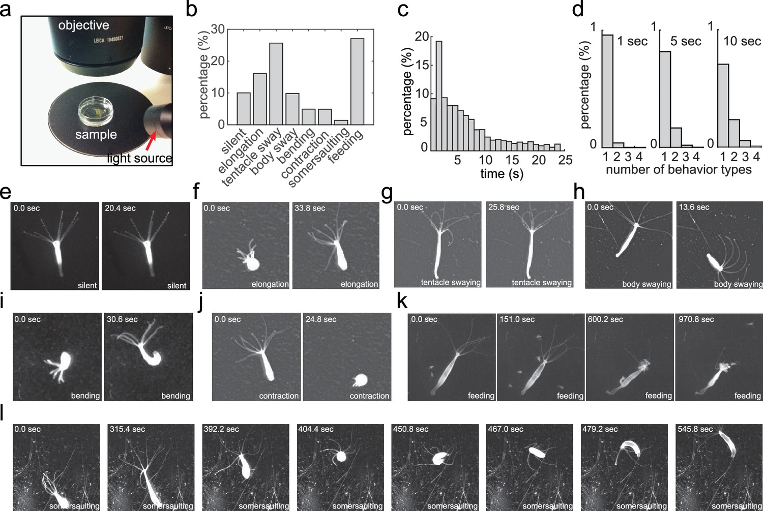
Acquiring an annotated Hydra behavior dataset.
(a) Imaging Hydra behavior with a widefield dissecting microscope. A Hydra polyp was allowed to move freely in a Petri dish, which was placed on a dark surface under the microscope objective. The light source was placed laterally, creating an bright image of the Hydra polyp on a dark background. (b) Histogram of the eight annotated behavior types in all data sets. (c) Histogram of the duration of annotated behaviors. (d) Histogram of total number of different behavior types in 1 s, 5 s and 10 s time windows. (e–l) Representative images of silent (e), elongation (f), tentacle swaying (g), body swaying (h), bending (i), contraction (j), feeding (k), and somersaulting (l) behaviors.
Figure 1—figure supplement 1
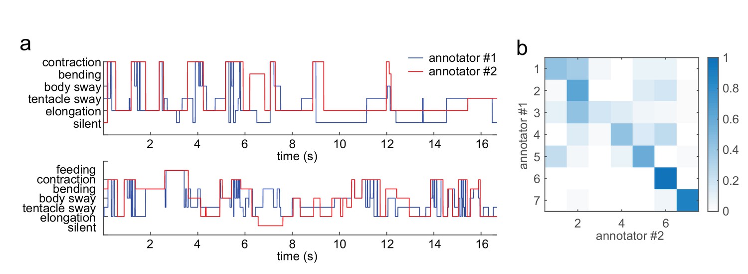
Variability of human annotators.
(a) Two example segments of annotations from two different human annotators. (b) Confusion matrix of the two annotations from four representative behavior videos. The overall match is 52%.
Figure 2 with 1 supplement
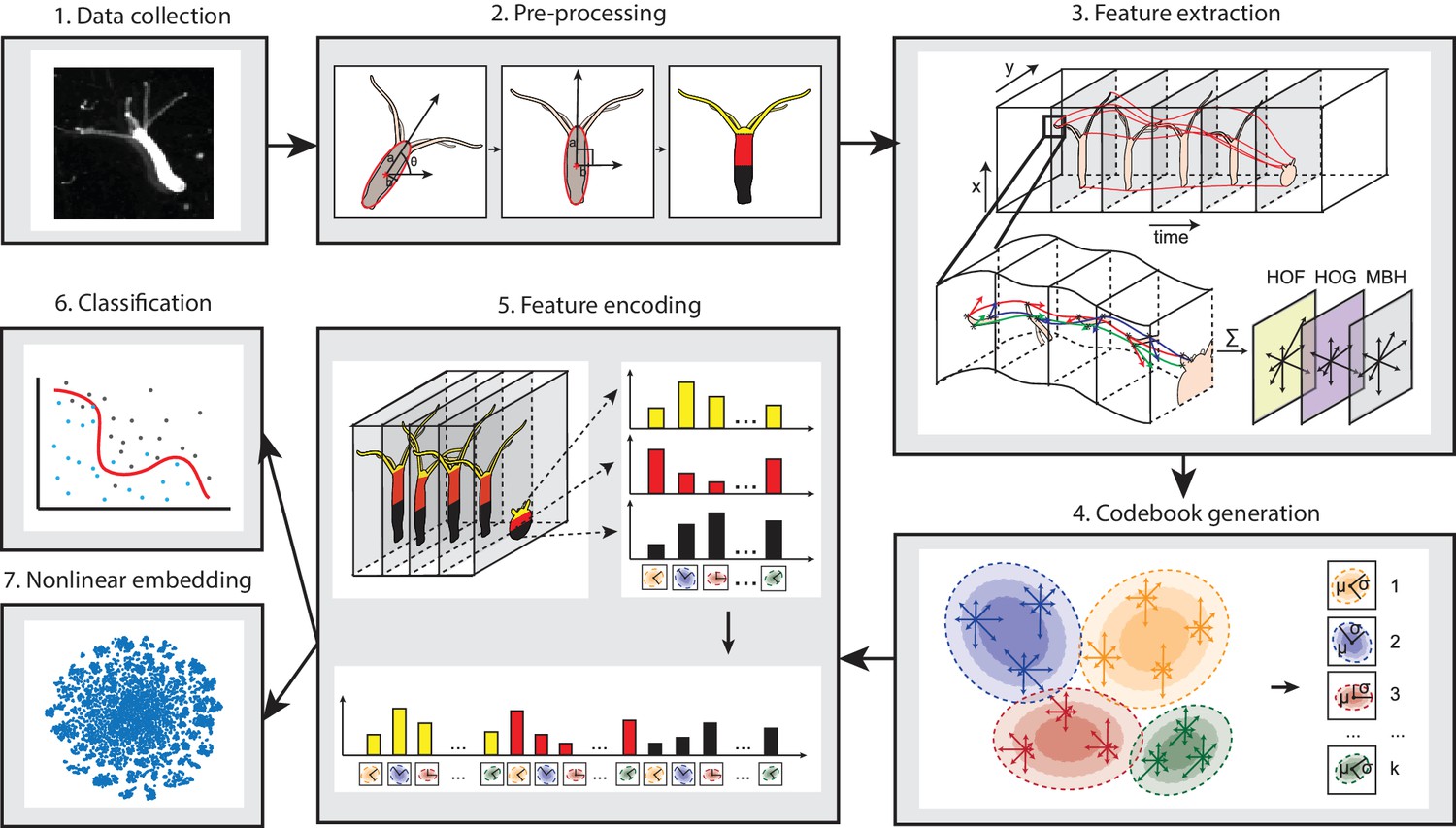
Analysis pipeline.
Videos of freely moving Hydra polyps were collected (1), then, Hydra images were segmented from background, and the body column was fit to an ellipse. Each time window was then centered and registered, and the Hydra region was separated into three separate body parts: tentacles, upper body column, and lower body column (2). Interest points were then detected and tracked through each time window, and HOF, HOG and MBH features were extracted from local video patches of interest points. Gaussian mixture codebooks were then generated for each features subtype (4), and Fisher vectors were calculated using the codebooks (5). Supervised learning using SVM (6), or unsupervised learning using t-SNE embedding (7) was performed using Fisher vector representations.
Figure 2—figure supplement 1
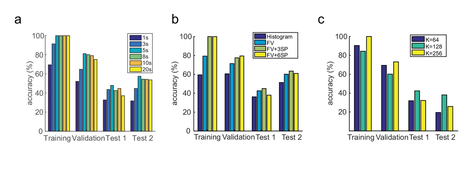
Model and parameter selection.
(a) Classification performance using time windows of 1, 3, 5, 8, 10 and 20 s, on training, validation and two test data sets. (b) Classification performance with normalized histogram representation, Fisher Vector (FV) representation, Fisher Vector with three spatial body part segmentation (3SP), Fisher Vector with six spatial body part segmentation (6SP), on training, validation and two test data sets. (c) Classification performance with K = 64, 128 and 256 Gaussian Mixtures for FV encoding, on training, validation and two test data sets.
Figure 3
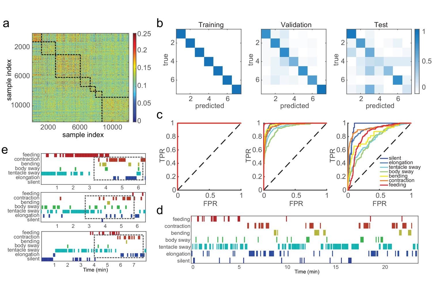
SVM classifiers recognize pre-defined Hydra behavior types.
(a) Pairwise Euclidean similarity matrix of extracted Fisher vectors. Similarity values are indicated by color code. (b) Confusion matrices of trained classifiers predicting training, validation, and test data. Each column of the matrix represents the number in a predicted class; each row represents the number in a true class. Numbers are color coded as color bar indicates. (Training: n = 50, randomly selected 90% samples; validation: n = 50, randomly selected 10% samples; test: n = 3) (c) ROC curves of trained classifiers predicting training, validation and test data. TPR, true positive rate; FPR, false positive rate. Dashed lines represent chance level. (d) An example of predicted ethogram using the trained classifiers. (e) Three examples of SVM classification of somersaulting behaviors. Dashed boxes indicate the core bending and flipping events.
Figure 4 with 1 supplement
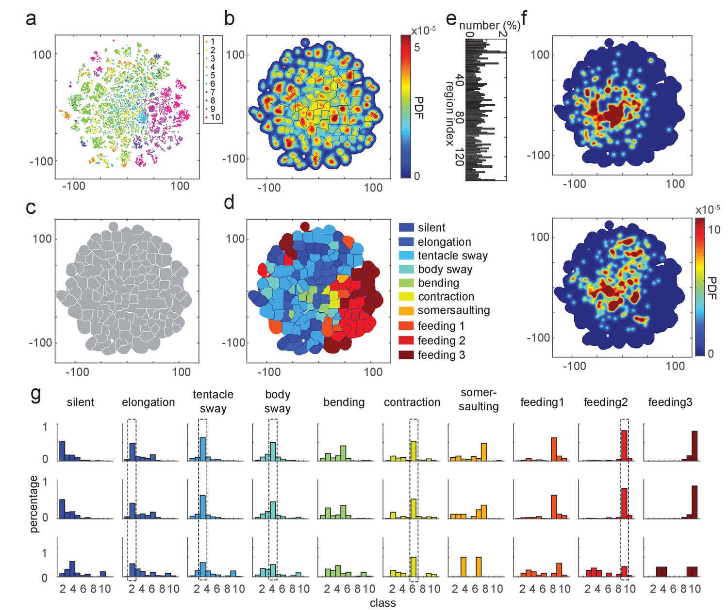
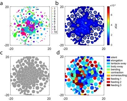
t-SNE embedding map of behavior types.
(a) Scatter plot with embedded Fisher vectors. Each dot represents projection from a high-dimensional Fisher vector to its equivalent in the embedding space. Color represents the manual label of each dot. (b) Segmented density map generated from the embedding scatter plot. (c) Behavior motif regions defined using the segmented density map. (d) Labeled behavior regions. Color represents the corresponding behavior type of each region. (e) Percentage of the number of samples in each segmented region. (f) Two examples of embedded behavior density maps from test Hydra polyps that were not involved in generating the codebooks or generating the embedding space. (g) Quantification of manual label distribution in training, validation and test datasets. Dashed boxes highlight the behavior types that were robustly recognized in all the three datasets. Feeding 1, the tentacle writhing or the first stage of feeding behavior; feeding 2, the ball formation or the second stage of feeding behavior; feeding 3, the mouth opening or the last stage of feeding behavior.
Figure 4—figure supplement 1
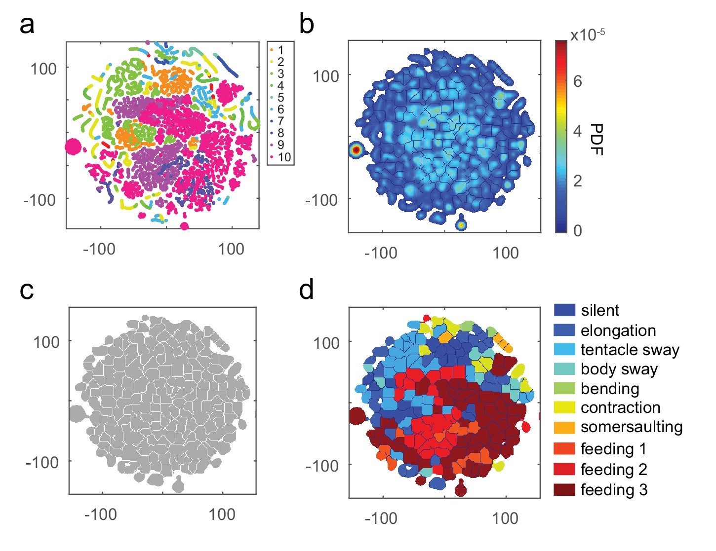
t-SNE embedding of continuous time windows.
(a) Scatter plot with embedded Fisher vectors. Each dot represents projection from a high-dimensional Fisher vector to its equivalent in the embedding space. The Fisher vectors were encoded from continuous 5 s windows with an overlap of 24 frames. Color represents the manual label of each dot. (b) Segmented density map generated from the embedding scatter plot. (c) Behavior motif regions defined using the segmented density map. (d) Labeled behavior regions with manual labels. Color represents the corresponding behavior type of each region.
Figure 5

t-SNE embedding reveals unannotated egestion behavior.
(a) Experimental design. A Hydra polyp was imaged for 3 days and nights, with a 12 hr light/12 hr dark cycle. (b) A Hydra polyp was imaged between two glass coverslips separated by a 100 µm spacer. (c) Left: density map of embedded behavior during the 3-day imaging. Right: segmented behavior regions with the density map. Magenta arrow indicates the behavior region with discovered egestion behavior. (d) Identification of egestion behavior using width profile. Width of the Hydra polyp (gray trace) was detected by fitting the body column of the animal to an ellipse, and measuring the minor axis length of the ellipse. The width trace was then filtered by subtracting a 15-minute mean width after each time point from a 15-minute mean width before each time point (black trace). Peaks (red stars) were then detected as estimated time points of egestion events (Materials and methods). (e) Density of detected egestion behaviors in the embedding space. Magenta arrow indicates the high density region that correspond to the egestion region discovered in c.
Figure 6
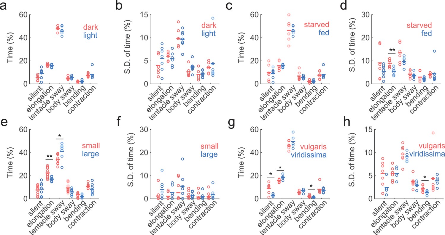
Similar behavior statistics under different conditions but differences across species.
(a) Percentage of time Hydra spent in each behavior, in dark (red to infra-red) and light conditions. Each circle represents data from one individual. The horizontal line represents the average of all samples. Red represents dark condition, blue represents light condition. (ndark = 6, nlight = 7) (b) Standard deviations of behaviors within each individual animal, calculated with separate 30 min time windows in the recording. Each circle represents the behavior variability of one individual. (c) Percentage of time Hydra spent in each behavior, in starved and well-fed condition. (nstarved = 6, nfed = 7) (d) Standard deviations of individual behaviors under starved and well-fed conditions. (e) Percentage of time small and large Hydra spent in each behavior. (nsmall = 10, nlarge = 7). (f) Standard deviations of behaviors of small and large individuals. (g) Percentage of time Hydra vulgaris and Hydra viridissima spent in each behavior type. (nvulgaris = 7, nviridissima = 5). (h) Standard deviations of individual brown and green Hydra. *p<0.05, **p<0.01, Wilcoxon rank-sum test.
Author response image 1
t-SNE embedding of continuous time windows.
a, Scatter plot with embedded Fisher vectors from 50 Hydra. Each dot represents projection from a high-dimensional Fisher vector to its equivalent in the embedding space. The Fisher vectors were encoded from continuous 5-second windows with an overlap of 24 frames. Color represents the manual label of each dot. b, Segmented density map generated from the embedding scatter plot. c, Behavior motif regions defined using the segmented density map. d, Labeled behavior regions with manual labels. Color represents the corresponding behavior type of each region.
Videos
Video 1
Example of elongation behavior.
The animal was allowed to move freely in a petri dish. The video was taken at 5 Hz, and was accelerated 20 fold.
Video 2
Example of tentacle swaying behavior.
The animal was allowed to move freely in a petri dish. The video was taken at 5 Hz, and was accelerated 20 fold.
Video 3
Example of body swaying behavior.
The animal was allowed to move freely in a petri dish. The video was taken at 5 Hz, and was accelerated 20 fold.
Video 4
Example of bending behavior.
The animal was allowed to move freely in a petri dish. The video was taken at 5 Hz, and was accelerated 20 fold.
Video 5
Example of a contraction burst.
The animal was allowed to move freely in a petri dish. The video was taken at 5 Hz, and was accelerated 20 fold.
Video 6
Example of induced feeding behavior.
The animal was treated with reduced L-glutathione at 45 s. The video was taken at 5 Hz, and was accelerated 20 fold.
Video 7
Example of somersaulting behavior.
The video was taken at 5 Hz, and was accelerated by 20 fold.
Video 8
Example of the output of body part segmentation.
White represents tentacle region, yellow represents upper body column region, and red represents lower body column region.
Video 9
Examples of detected interest points (red) and dense trajectories (green) in tentacle swaying (left), elongation (middle left), body swaying (middle right), and contraction (right) behaviors in 2 s video clips.
Upper panels show the original videos; lower panels show the detected features.
Video 10
Example of the trained SVM classifiers predicting new data.
https://doi.org/10.7554/eLife.32605.018
Video 11
Example of the trained SVM classifiers predicting somersaulting behavior from a new video.
Soft prediction was allowed here.
Video 12
Examples from the identified silent region in the embedding space.
https://doi.org/10.7554/eLife.32605.023
Video 13
Examples from the identified slow elongation region in the embedding space.
https://doi.org/10.7554/eLife.32605.024
Video 14
Examples from the identified fast elongation region in the embedding space.
https://doi.org/10.7554/eLife.32605.025
Video 15
Examples from the identified inter-contraction elongation region in the embedding space.
https://doi.org/10.7554/eLife.32605.026
Video 16
Examples from the identified bending region in the embedding space.
https://doi.org/10.7554/eLife.32605.027
Video 17
Examples from the identified tentacle swaying region in the embedding space.
https://doi.org/10.7554/eLife.32605.028
Video 18
Examples from the identified initial contraction region in the embedding space.
https://doi.org/10.7554/eLife.32605.029
Video 19
Examples from the identified contracted contraction region in the embedding space.
https://doi.org/10.7554/eLife.32605.030
Video 20
Examples from the identified egestion region in the embedding space.
https://doi.org/10.7554/eLife.32605.031
Video 21
Examples from the identified hypostome movement region in the embedding space.
https://doi.org/10.7554/eLife.32605.032Tables
Table 1
SVM statistics. AUC: area under curve; Acc: accuracy; Prc: precision; Rec: recall.
https://doi.org/10.7554/eLife.32605.017| Behavior | Train | Withheld | Test | |||||||||||||||
|---|---|---|---|---|---|---|---|---|---|---|---|---|---|---|---|---|---|---|
| AUC | AUC chance | Acc | Acc chance | Prc | Rec | AUC | AUC chance | Acc | Acc chance | Prc | Rec | AUC | AUC chance | Acc | Acc chance | Prc | Rec | |
| Silent | 1 | 0.5 | 100% | 9.6% | 100% | 100% | 0.98 | 0.5 | 95.6% | 9.6% | 75.6% | 97.4% | 0.95 | 0.5 | 90.3% | 1.9% | 18.4% | 90.3% |
| Elongation | 1 | 0.5 | 100% | 14.2% | 100% | 100% | 0.96 | 0.5 | 93.4% | 13.6% | 76.4% | 95.9% | 0.91 | 0.5 | 87.9% | 22.2% | 71.4% | 92.6% |
| Tentacle sway | 1 | 0.5 | 100% | 25.1% | 100% | 100% | 0.95 | 0.5 | 89.6% | 25.0% | 77.5% | 92.4% | 0.76 | 0.5 | 71.9% | 30.2% | 47.9% | 76.7% |
| Body sway | 1 | 0.5 | 100% | 10.0% | 100% | 100% | 0.92 | 0.5 | 92.9% | 9.3% | 65.7% | 97.0% | 0.75 | 0.5 | 83.4% | 17.7% | 52.8% | 95.4% |
| Bending | 1 | 0.5 | 100% | 5.2% | 100% | 100% | 0.98 | 0.5 | 97.3% | 6.1% | 74.4% | 98.4% | 0.81 | 0.5 | 93.9% | 6.1% | 38.9% | 96.5% |
| Contraction | 1 | 0.5 | 100% | 6.6% | 100% | 100% | 0.97 | 0.5 | 95.7% | 6.9% | 70.4% | 97.7% | 0.92 | 0.5 | 92.8% | 11.7% | 63.2% | 95.5% |
| Feeding | 1 | 0.5 | 100% | 29.2% | 100% | 100% | 1 | 0.5 | 98.8% | 29.6% | 98.5% | 99.4% | 0.83 | 0.5 | 81.0% | 10.2% | 39.6% | 94.1% |
Download links
A two-part list of links to download the article, or parts of the article, in various formats.
Downloads (link to download the article as PDF)
Open citations (links to open the citations from this article in various online reference manager services)
Cite this article (links to download the citations from this article in formats compatible with various reference manager tools)
Comprehensive machine learning analysis of Hydra behavior reveals a stable basal behavioral repertoire
eLife 7:e32605.
https://doi.org/10.7554/eLife.32605


