Why plants make puzzle cells, and how their shape emerges
- Max Planck Institute for Plant Breeding Research, Germany
- University of Calgary, Canada
- Indian Institute of Science, India
- Cornell University, United States
- Université de Lyon, ENS de Lyon, UCBL, INRA, CNRS, France
- Stockholm University, Sweden
Figures
Figure 1

Relationship between cell shape and stress.
(A) Cell contours in adaxial epidermis of an Arabidopsis thaliana cotyledon. Small, elliptical cells are stomata. Scale bar: 50 µm. (B–F) Cellular stress patterns in finite element method (FEM) simulations. Cell walls have uniform, isotropic material properties (Young's modulus = 300 MPa) and are inflated to the same turgor pressure (5 bar). (B) Graph points show stress in cells expanded in one dimension (circles), two dimensions (stars) or three dimensions (triangles). Enlargement in two or more dimensions substantially increases stress in the center of the cell walls. (C) Principal stresses generated by turgor in vivo were simulated in a FEM model on a template extracted from confocal data. (D) A simplified tissue template using the junctions of the cells in (C). The yellow outline marks a corresponding cell in (C) and (D). Total area and number of cells is the same, however the maximal stress is much lower in the puzzle-shaped cells compared to the more isodiametrically-shaped cells. (E) In isolated circular cells, pressure-induced stress increases with diameter (triangles), as was the case in (B). Adding lobes, regardless of their length, width or number (inset) does not influence maximal stress in the cell wall in the center (stars). (F) A close-up view showing high stress areas that coincide with the center of the large open area of the cell, or indentations that support large open areas. (G) Measures used to quantify puzzle cell shape and stress. The largest empty circle (LEC, yellow) that fits inside the cell is a proxy for the maximal stress in the cell wall. The convex hull (red) is the smallest convex shape that contains the cell. The ratio of cell perimeter (white) to the convex hull perimeter gives a measure of how lobed the cell is (termed ‘lobeyness’). Scale bars: 50 µm (C,D), 10 µm (F). Color scale: trace of Cauchy stress tensor in MPa.
Figure 2 with 1 supplement
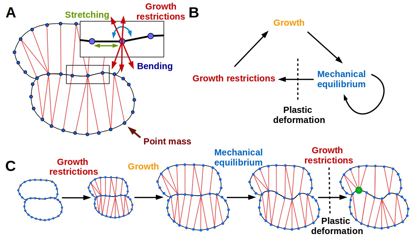
The 2D puzzle cell model.
(A) Mechanical representation of cells. Cell walls are discretized into a sequence of point masses (blue circles) connected by linear wall-segments (black lines). Growth restricting connections (red lines) join point masses across the cell. The forces acting on the point mass are produced by stretching of wall segments and growth restricting connections as well as bending of the cell wall at the mass. (B–C) The simulation loop consists of 3 steps (B), as depicted for a diagrammatic example in (C). Step 1: additional transversal springs (red) are added to the model to represent oriented cell wall stiffening components guided by microtubules connecting opposing sides of the cell. They act like one-sided springs, in that they exert a force when under tension (i.e. stretched beyond their rest length), but are inactive when compressed. This is consistent with the high tensile strength of cellulose. Step 2: the tissue is scaled to simulate growth, which can have a preferred direction (i.e. is anisotropic). Step 3: the network of springs reaches mechanical equilibrium. Transversal springs restrict cell expansion in width, causing cell walls to bend. Before the next iteration, wall springs are relaxed and transversal springs are rearranged to reflect the new shape of cells. Cell shapes emerging in the model are determined by the nature of the assumed tissue growth direction. Note that in (C) the deformation of the cell causes the placement of growth restrictions to change during the subsequent iteration, where the green mass at the lobe tip attracts more connections on the convex side and loses connections on the concave side (in line with the model assumption of not restricting growth in concave regions).
Figure 2—figure supplement 1
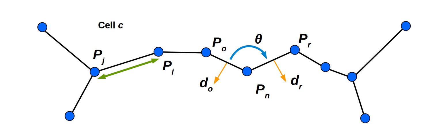
Mechanical properties of the cell wall are simulated using stretching and bending springs.
See Appendix Mechanical simulation for details. The linear spring connecting masses mi and mj is shown, and generates a force parallel to the line connecting their positions Pi and Pj (green line with arrowheads). The bending spring in cell c at mass mn generates a force acting on mn and the neighboring masses mo and mr. The sign and magnitude is determined by θ (the signed angle between Po and Pr). The vector do (the outward facing normal to the cell wall spanning Pn and Po) determines the direction of the force acting on mass mo. The vector dr is defined similarly, and determines the direction of the force acting on mr. The force acting on mass mn balances those acting on masses mo and mr.
Figure 3 with 2 supplements
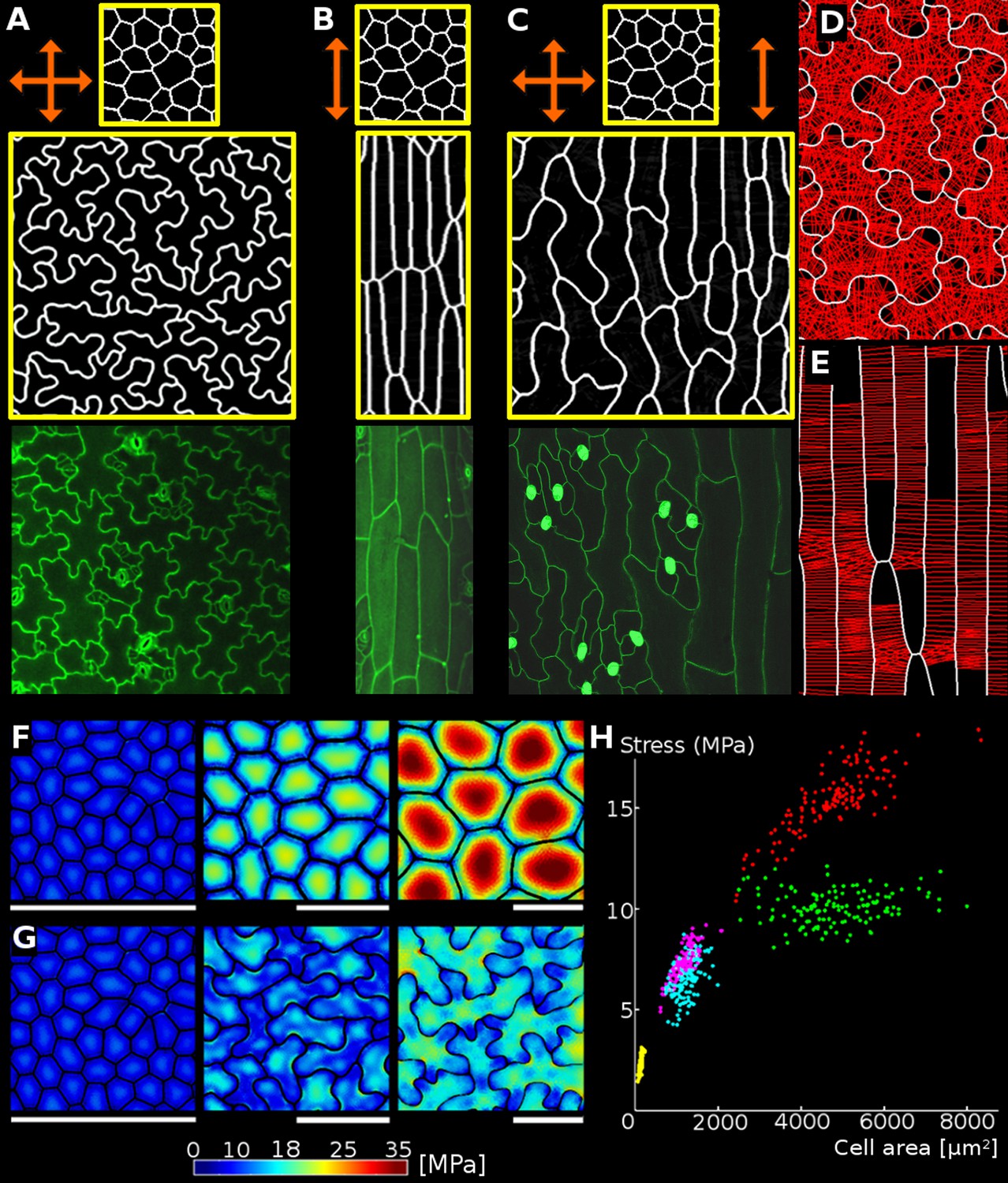
Geometric-mechanical model of puzzle cell emergence.
(A) Starting with meristematic-like cells (top), growing the tissue isotropically, i.e. equally in all directions (arrows), produces puzzle-shaped cells (middle) that resemble cotyledon epidermal cells (bottom). (B) Growing the tissue primarily in one direction (anisotropically) results in elongated cells (middle) as observed, for example, in the petiole (bottom). (C) A gradient of growth anisotropy (increasing left to right) produces a spatial gradient of cell shapes (middle), as observed between the blade and midrib of a leaf (bottom). (D–E) Connections of transversal springs (red) restricting growth in each simulation step in tissues with isotropic (D) and anisotropic (E) growth. To make connections more apparent, only 50% are visualized. (F–G) Cell outlines from 2D models with isotropic growth were used to generate 3D templates for FEM models (growth progresses from left to right, scale bars: 80 µm). (F) As the tissue grows, cells lacking transversal springs conserve their original shape. In pressurized cells, mechanical stress increases with the cell size. (G) When transversal springs are added, tissue expansion generates lobed cells. (H) Average stress in the cell increases with cell area in the polygonal cells (yellow, pink, red), while stress plateaus during tissue grows when cells form lobes (cyan, green). Points of each color represent cells of increasing size, with stresses calculated using the FEM model. Color scale: trace of Cauchy stress tensor in MPa.
Figure 3—figure supplement 1
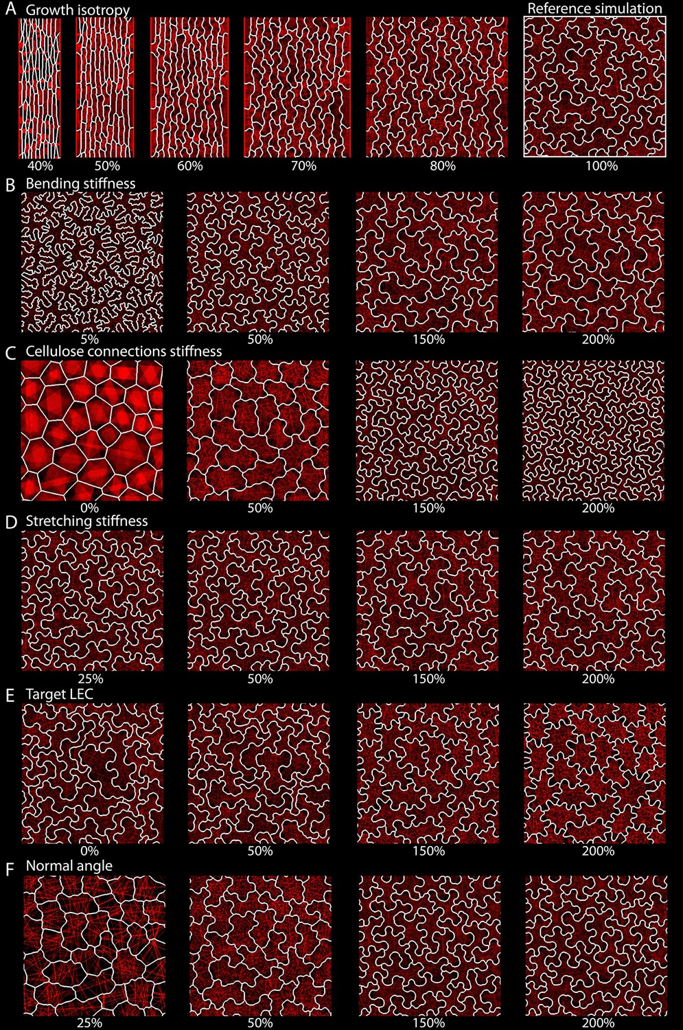
Parameter space exploration for key model parameters.
The wild type isotropic simulation was used as the reference simulation (A, 100%), and parameters were varied independently. Isotropy was varied from 40% to 100% of the reference value and all other parameters were varied from (at least) 25% to 200%. Snapshots of the final stage of each simulation are displayed. The varied parameters were: (A) growth isotropy (growth in width vs growth in length), (B) bending stiffness, (C) cellulose connection stiffness, (D) stretching stiffness, (E) target LEC, (F) normal angle.
Figure 3—figure supplement 2
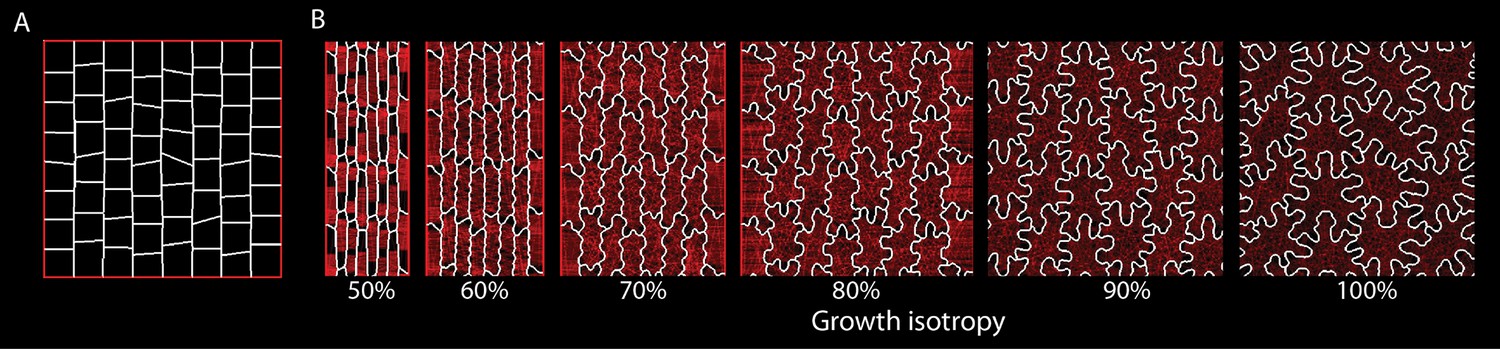
Varying isotropy for an alternative parameter set.
Using a different parameter set compared to Figure 3—figure supplement 1A, growth isotropy was varied while all other parameters were constant. Compared to Figure 3—figure supplement 1A, target LEC has been increased by 100%, simulation time extended by 10%, and the initial cellular template was changed to that shown in (A). (B) Snapshots of the final stage of each simulation as isotropy (growth in width vs growth in length) was varied from 50% to 100% Although cell morphology changes, the relation between isotropy and puzzle-cell development is maintained.
Figure 4 with 1 supplement

Correlation between growth direction and shape on the cell and organ level.
(A-B) Time-lapse confocal imaging. Pictures were taken every 48 hr and analyzed using MorphoGraphX. The last time point of each series is shown. Growth anisotropy between 2 and 6 days after germination (DAG), calculated as the expansion rate in the direction of maximal growth divided by expansion rate in the direction of minimal growth, and cell lobeyness in wildtype (A) and p35S::LNG1 (B) cotyledons. The p35S::LNG1 cotyledon displays more anisotropic growth and less lobed epidermal cells. Scale bars: 50 µm. (C-E) p35S::LNG1 T1 plants with wild type-like phenotype (C, 61/98 plants), strong phenotype with dramatically elongated cotyledons and leaves (D, 16/98 plants) and intermediate phenotype with elongated cotyledons but wt-like leaves (E, 12/98 plants). Cotyledons are marked by white dots. The remaining nine obtained plants displayed elongated costyledons and mildly elongated leaves (not shown). (F-I) Confocal images of epidermal cells. Scale bars: 20 µm. (F) shows cells from a leaf in (C), (G) shows cells from a leaf in (D), (H) shows cells from a cotyledon in (E), and (I) shows cells from a leaf in (E). (J-K) Epidermal cell outlines from fruit with more isotropic shapes (silicles, J) and more anisotropic shapes (siliques, K).Fruit images reproduced from Figure 4 and S4 of Hofhuis et al., 2016; published under the terms of the Creative Commons Attribution license (http://creativecommons.org/licenses/by/4.0/). Cell outlines reproduced from Figure 2 of Hofhuis and Hay (2017), adapted with permission from John Wiley and Sons. Scale bars: 10 µm for cell outlines, 1 mm for fruit. (L) Depolymerization of cortical microtubules by oryzalin treatment causes cells of NPA-treated meristems to expand without division, ultimately leading to the rupture of the cell wall due to increased mechanical stress. Regions where cells have ruptured (white stars) are primarily located on the flanks of the meristems, where cells are larger. Scale bar: 20 µm.
Figure 4—figure supplement 1
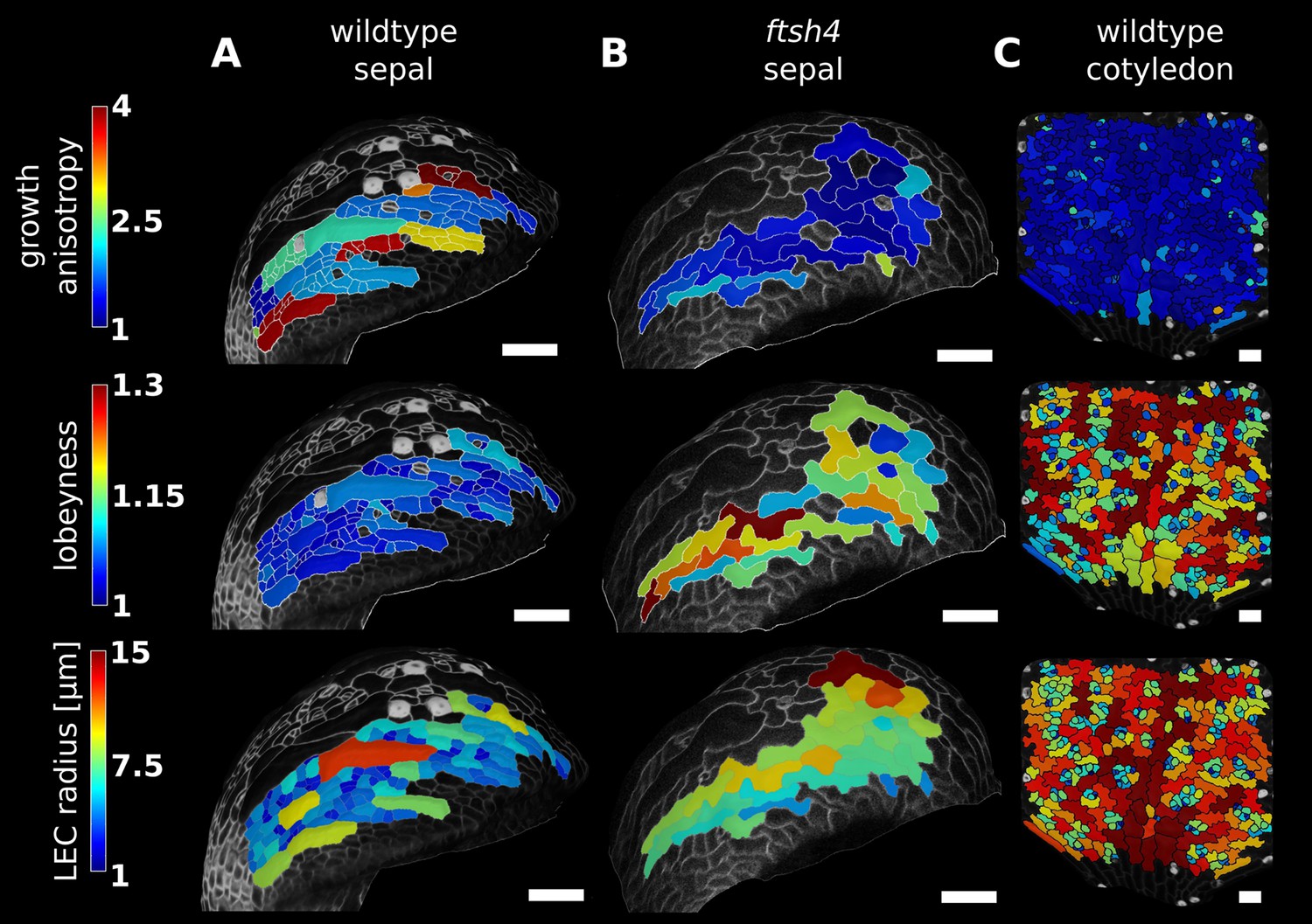
Correlation between growth direction and shape on the cell and organ level demonstrated by time-lapse confocal imaging.
Pictures were taken at 24 hr intervals for 3 days (A, wild type sepal; B, ftsh4 sepal) or 2 days (C, wild type cotyledon) and analyzed using MorphoGraphX. The last time point of each series is shown. Characterization of growth anisotropy (expansion rate in the direction of maximal growth divided by expansion rate in direction of minimal growth) and cell shape (lobeyness and LEC radius) in wildtype sepal, ftsh4 sepal and the wild type cotyledon, scale bars: 50 µm. Growth patterns of the wild type and ftsh4 sepals shown were previously described in (Hervieux et al., 2016) and (Hong et al., 2016), respectively.
Figure 5 with 3 supplements
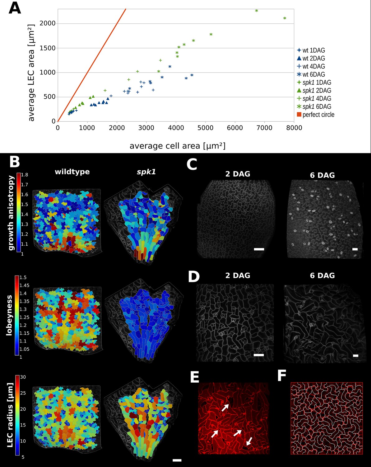
Characterization of spike1 mutant.
(A) Average LEC area of wild type and spk1 cotyledons vs. average cell area. The red line represents the theoretical case of a perfectly circular cell. In this case cell area and LEC area increase at the same rate. For the cell area and the LEC area analysis we considered the average values for the largest 20% of segmented cells in order to avoid bias stemming from the much smaller cells of the stomatal lineage, which due to their small size would not need to regulate their LEC. For average values for each point, including sample size and SE, see Figure 5—source data 1. (B) Time-lapse data on wild type and spk1 cotyledons. Plants were imaged twice in 48 hr intervals. Heat maps are displayed on the last time points. Scale bar: 100 µm. (C and D) Examples of cell shapes in the experiment shown in (A). Scale bars: 50 µm. (C) Wild type. (D) spk1. (E) Confocal image of spk1 cotyledon, 8 DAG. Note the gaps between cells and ruptured stomata that typify spk1 phenotype (arrows indicate several examples). (F) Model result with placement of transverse connections in lobe tips combined with parameter changes to account for defects in ROP-mediated cytoskeletal rearrangement (see main text).
-
Figure 5—source data 1
Average cell area and LEC area for wt and spk1 cotyledon time-course.
This table contains average values for 20% largest segmented cells (in each sample), displayed in Figure 5A.
- https://doi.org/10.7554/eLife.32794.024
-
Figure 5—source data 2
Mean average cell area for wild type and spk1 cotyledon cells (20% largest segmented cells for each sample, averaged), displayed in Figure 5—figure supplement 3.
- https://doi.org/10.7554/eLife.32794.025
Figure 5—figure supplement 1
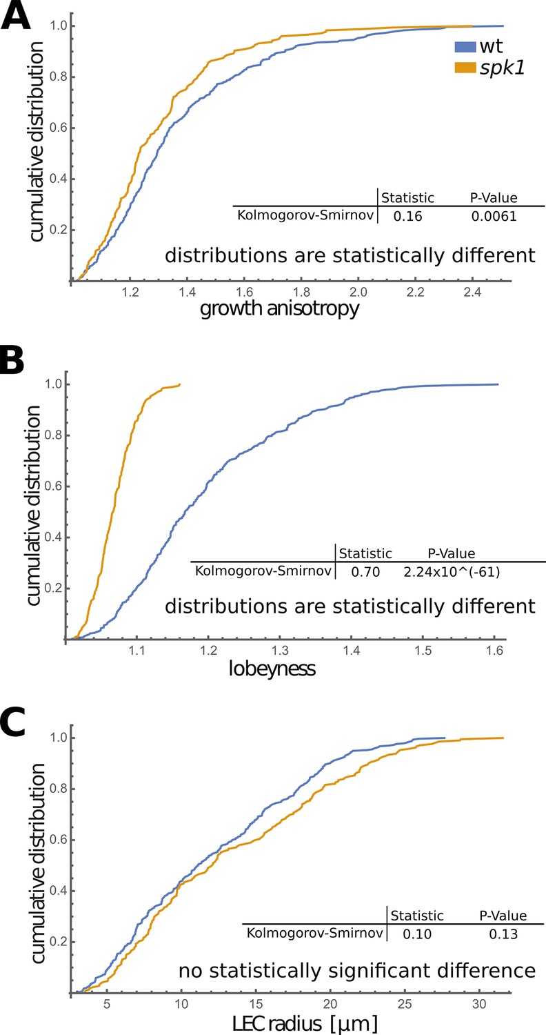
Comparison of growing wt and spk1 cotyledons.
Cumulative distribution of growth anisotropy (A), lobeyness (B) and LEC radius (C) of cells of wild type and spk1 cotyledons. A Kolmogorov-Smirnov test performed on data from time-lapse imaging experiments (Figure 5B) showed that growth anisotropy and cell lobeyness are statistically different in spk1 compared to wild type (A, B), while there is no statistically significant difference of LEC radius distribution between the two genotypes (C). We consider two distributions different if the p-value is higher than 0.05. This suggests that cells arrive at similar mechanical stress levels (here represented by LEC size) in different ways.
Figure 5—figure supplement 2
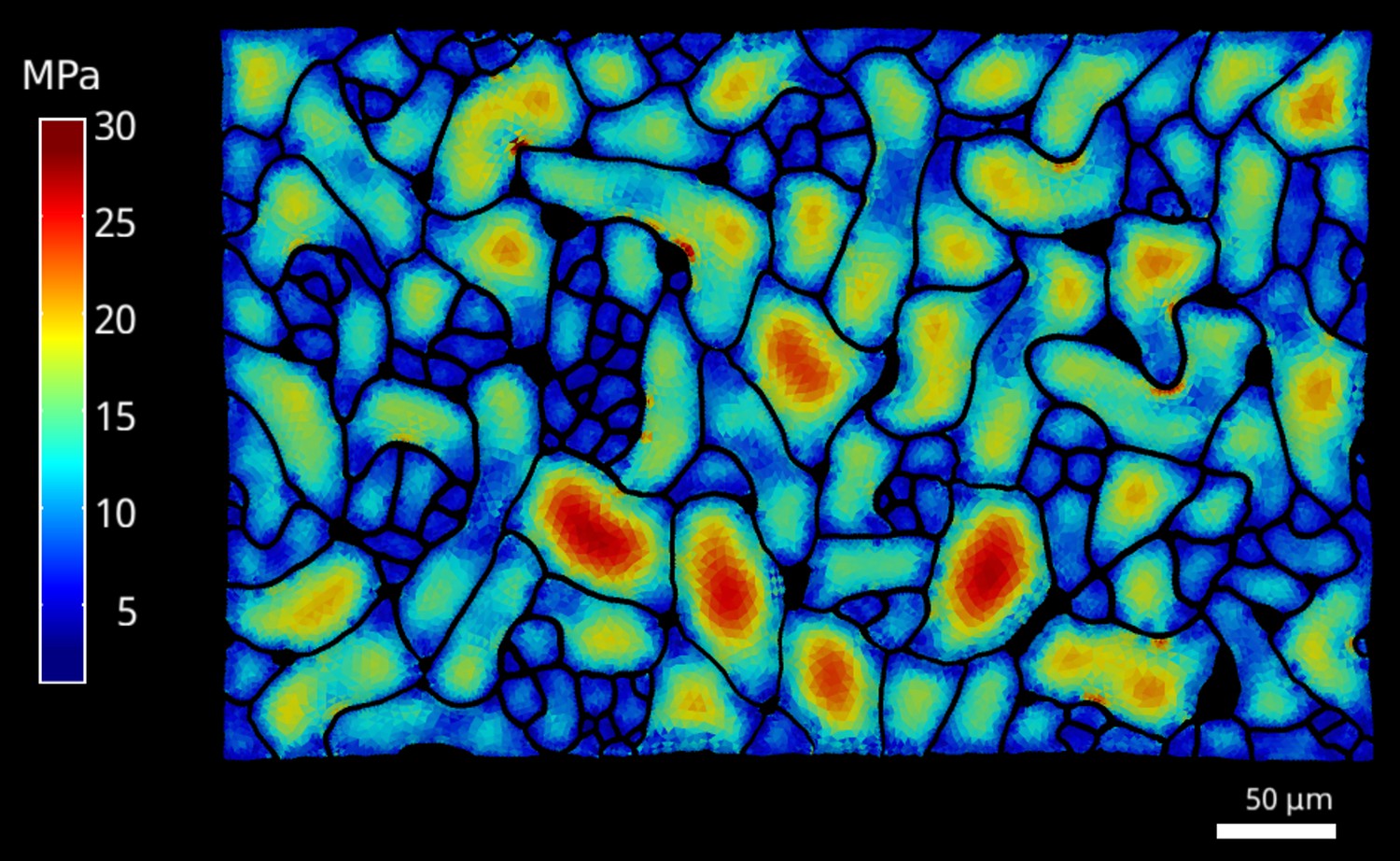
Cellular stress patterns in spike1 cells.
The FEM simulations were performed as described for the data in Figure 1, using spike1 epidermal cells. Color scale: trace of Cauchy stress tensor in MPa.
Figure 5—figure supplement 3
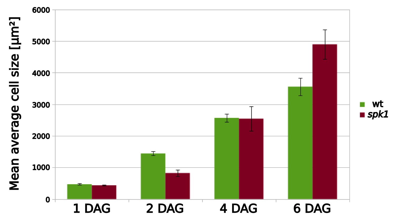
Mean average cell area for wild type and spk1 cells.
Data obtained from the data displayed in Figure 5A. For mean average values including SE, please see Figure 5—source data 2.
Figure 6
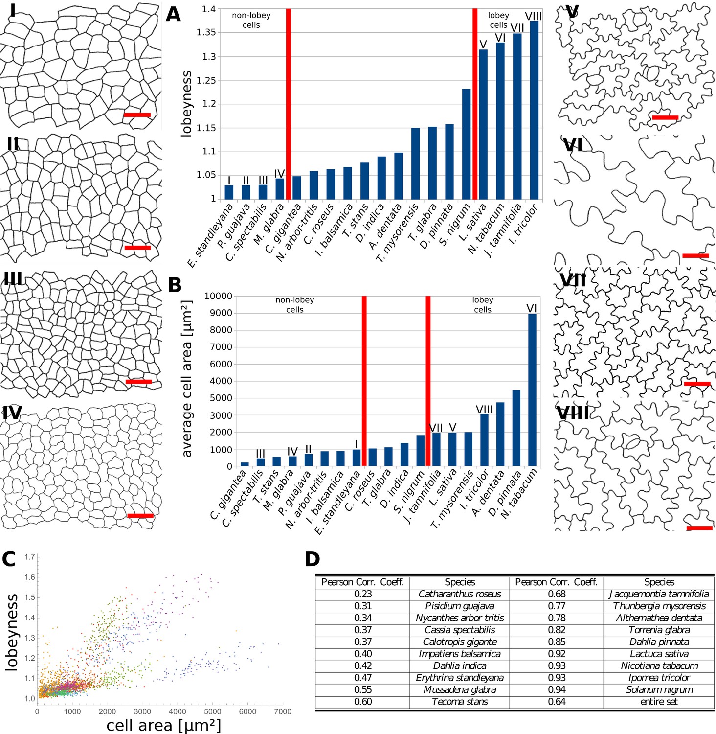
Multi-species cell shape analysis.
(A) Average cell lobeyness. (B) Average cell area. (I-VIII) Pictures of leaf epidermal cells of species corresponding to numbering in (A) and (B), numbered by the order of appearance in (A). Scale bars, 50 µm. (C) A plot of lobeyness vs. area for cells of all species pooled together. Each color symbolizes one species. (D) Pearson correlation coefficients between lobeyness and cell area for each species and for all cells pooled together (entire set). Note that in all cases a positive correlation between lobeyness and cell area is observed (correlation coefficient is greater than 0).
-
Figure 6—source data 1
Average cell area and lobeyness for all studied species.
Number of cells measured for each species, average values and SE are included. Figure supplements (captions embedded in the text alongside primary figures).
- https://doi.org/10.7554/eLife.32794.028
Appendix 1—figure 1
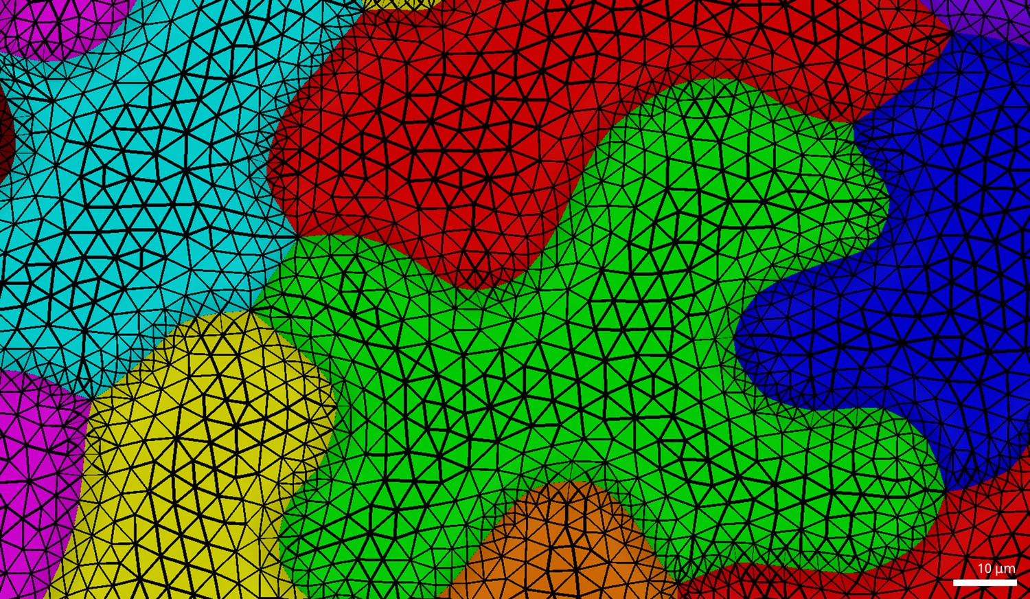
Pavement cell triangulation used in FEM simulations (Figure 1).
Note the smooth gradient of triangle sizes from the cell center towards its margin.
Videos
Video 1
Simulation of cell shape development in an isotropically expanding tissue.
The tissue is shown at two scales: unscaled (Left) and scaled to maintain a constant tissue width (Right). Red lines traversing cell-interiors correspond to active growth restrictions. Scale bar indicates a constant reference length.
Video 2
Simulation of cell shape development in an anisotropically expanding tissue.
The tissue is shown at two scales. (Left) Scaled to maintain a constant tissue width. (Right) Scaled so that the largest dimension of the tissue is constant. Scale bars indicate a common constant reference length.
Video 3
Simulation of cell shape development in a non-uniformly expanding tissue.
Growth anisotropy increases linearly from left to right. The tissue is shown at two scales: unscaled (Left) and scaled to maintain a constant tissue width (Right). Red lines traversing cell interiors correspond to active growth restrictions. Scale bar indicates a constant reference length.
Video 5
Simulation results when growth isotropy is varied.
Using the wild type isotropic simulation as a reference, growth isotropy (growth in width/growth in height, or gx/gy in Appendix) is varied from 50% to 100% of the reference value in regular increments. Successive frames show the final stage of each simulation as isotropy is increased. Scale bars indicate a constant reference length.
Video 6
Simulation results when bending stiffness is varied.
Using the wild type isotropic simulation as a reference, bending stiffness (kb in Appendix) is varied with respect to the reference value from 5% to 25% and then from 25–200% by increments of 25%. Successive frames show the final stage of each simulation as the bending stiffness is increased. Scale bars indicate a constant reference length.
Video 7
Simulation results when cellulose stiffness is varied.
Using the wild type isotropic simulation as a reference, cellulose connections stiffness (km in Appendix) is varied with respect to the reference value from 0–200% by increments of 25%. Successive frames show the final stage of each simulation as the cellulose connections stiffness is increased. Scale bars indicate a constant reference length.
Video 8
Simulation results when stretching stiffness is varied.
Using the wild type isotropic simulation as a reference, stretching stiffness (ks in Appendix) is varied with respect to the reference value from 25–200% by increments of 25%. Successive frames show the final stage of each simulation as the stretching stiffness is increased. Scale bars indicate a constant reference length.
Video 9
Simulation results when target LEC is varied.
Using the wild type isotropic simulation as a reference, target LEC (minmicro in Appendix) is varied with respect to the reference value from 0–200% by increments of 25%. Successive frames show the final stage of each simulation as the target LEC is increased. Scale bars indicate a constant reference length.
Video 10
Simulation results when normal angle is varied.
Using the wild type isotropic simulation as a reference, normal angle (θmicro in Appendix) is varied with respect to the reference value from 25–200% by increments of 25%. Successive frames show the final stage of each simulation as the normal angle is increased. Scale bars indicate a constant reference length.
Video 4
Simulation of the development of spk1-like cells in an isotropically expanding tissue.
The tissue is shown at two scales: unscaled (Left) and scaled to maintain a constant tissue width (Right). Red lines traversing cell-interiors correspond to active growth restrictions. Scale bar indicates a constant reference length of arbitrary value.
Tables
Key resources table
| Reagent type (species) or resource | Designation | Source or reference | Identifiers | Additional information |
|---|---|---|---|---|
| gene | spk1 | Nottingham Arabidopsis Stock Centre | SALK_125206 | |
| gene | ftsh4-5 | Hong et al., 2016 | ||
| genetic reagent | p35S::LNG1 | this paper | Vector obtained using gateway cloning, transformed into Col-0 plants by Agrobacterium-mediated floral dipping | |
| genetic reagent | pUBQ10::myrYFP | Hervieux et al., 2016 | ||
| recombinant DNA reagent | LNG1CDS | this paper | Full-length CDS of LONGIFOLIA1 gene, PCR amplified | |
| recombinant DNA reagent | pENTR/D-TOPO | Invitrogen | ||
| recombinant DNA reagent | pK7WG2 | Karimi et al., 2002 | ||
| genetic reagent | p35S::LTI6b-GFP | Cutler et al., 2000 | ||
| other | N-(1-naphtyl) phtalamic acid (NPA) | Hamant et al., 2008 | ||
| other | oryzalin | Hamant et al., 2008 | ||
| software, algorithm | VVE | Smith et al., 2003 | www.algorithmicbotany.org | |
| software, algorithm | MorphoGraphX | Barbier de Reuille et al., 2015 | www.MorphoGraphX.org |
Appendix 1—table 1
Parameters for simulations of puzzle cell morphogenesis.
All simulations use the parameter values specified for isotropic growth (fourth column) unless otherwise specified.
| Parameter | Simulation | |||||
|---|---|---|---|---|---|---|
| Name | Symbol | Text reference | Isotropic growth | Anisotropic growth | Growth gradient | spk1 mutant |
| Initial width and height | Overview | 8.5 × 8.5 | 17 × 8.5 | 17 × 8.5 | ||
| Cell number | Overview | 128 | 256 | 256 | ||
| Edge subdivision threshold | Overview | 0.5 | ||||
| Growth step | Growth | 0.0075 | 0.015 | |||
| RERG along y-axis | Equation 1 | 1.25 | 1.0 | 1.5 | 1.5 | |
| RERG along x-axis (uniform growth) | Equation 1 | 1.25 | 0.35 | NA | 1.5 | |
| RERG along x-axis (non-uniform growth) | Equation 2 | [0.8,1.35] | ||||
| Maximum cell wall angle | Microtubule placement | |||||
| Cell wall tensional elastic modulus | Equation 7 | 0.4 | 2.0 | |||
| Bending spring constant | Equation 8-10 | 0.02 | 0.12 | |||
| Microtubular tensional elastic modulus | Equation 11 | 0.75 | 2.0 | |||
| Minimum active length | Equation 11 | 3 | ||||
| Maximum active length | Equation 11 | 300 | ||||
-
Microtubular connections can terminate in recessed portions of the cell-wall (i.e. condition 3 in Microtubule placement is ignored).
Additional files
-
Transparent reporting form
- https://doi.org/10.7554/eLife.32794.029
Download links
A two-part list of links to download the article, or parts of the article, in various formats.
Downloads (link to download the article as PDF)
Open citations (links to open the citations from this article in various online reference manager services)
Cite this article (links to download the citations from this article in formats compatible with various reference manager tools)
Why plants make puzzle cells, and how their shape emerges
eLife 7:e32794.
https://doi.org/10.7554/eLife.32794


