Post-decision biases reveal a self-consistency principle in perceptual inference
- University of Pennsylvania, United States
Figures
Figure 1 with 1 supplement
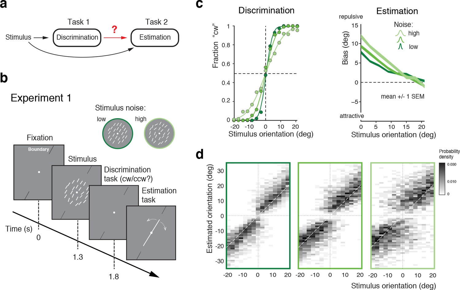
Post-decision biases in a perceptual task sequence.
(a) Perceptual decision-making in a discrimination-estimation task sequence: Does a discrimination judgment causally affect a subject’s subsequent perceptual estimate? (b) Experiment 1: After being presented with an orientation stimulus (array of lines), subjects first decided whether the overall array orientation was clockwise (cw) or counter-clockwise (ccw) of a discrimination boundary, and then had to estimate the actual orientation by adjusting a reference line with a joystick. Different stimulus noise levels were established by changing the orientation variance in the array stimulus. (c) Psychometric functions and estimation biases (combined subject). Estimation biases are only shown for correct trials and are combined across cw and ccw directions. Subjects show larger repulsive biases the noisier the stimulus and the closer the stimulus orientation was to the boundary. (d) Distributions of estimates for the three stimulus noise levels tested, plotted as a function of stimulus orientation relative to the discrimination boundary (combined subject). Estimates are clearly biased away from the discrimination boundary forming a characteristic bimodal pattern.
Figure 1—figure supplement 1
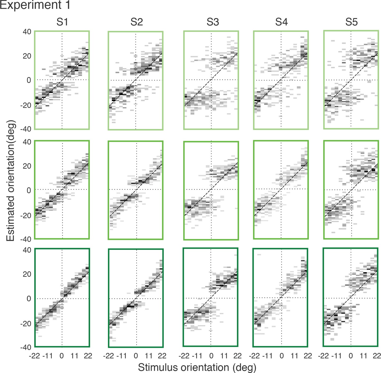
Full distributions of individual subjects’ estimates in Experiment 1.
Each row corresponds to one of the three stimulus noise conditions (color-code as in main text).
Figure 2
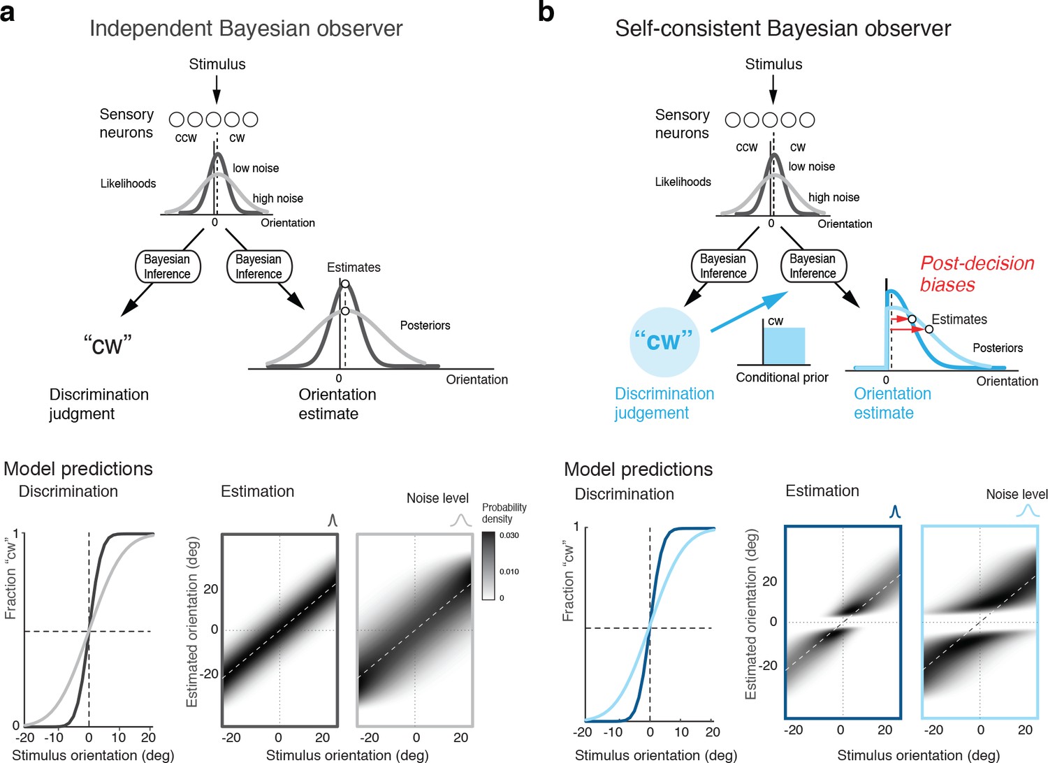
Bayesian observer models for the perceptual task sequence.
(a) The discrimination judgment does not affect the estimated stimulus orientation for an observer who considers both tasks independently. (b) In contrast, the self-consistent observer imposes a causal dependency such that the judgment in the discrimination task (e.g., 'cw’) conditions the estimation process in form of a choice-dependent prior. It effectively sets the posterior probability to zero for any orientation value that is inconsistent with the preceding discrimination judgment. The truncated posterior distribution, together with a loss function that penalizes larger estimation errors stronger than smaller ones, leads to the characteristic bimodal distribution pattern. Note, however, that this basic formulation is not quite sufficient to explain some details of the estimation data (Figure 1d).
Figure 3 with 2 supplements
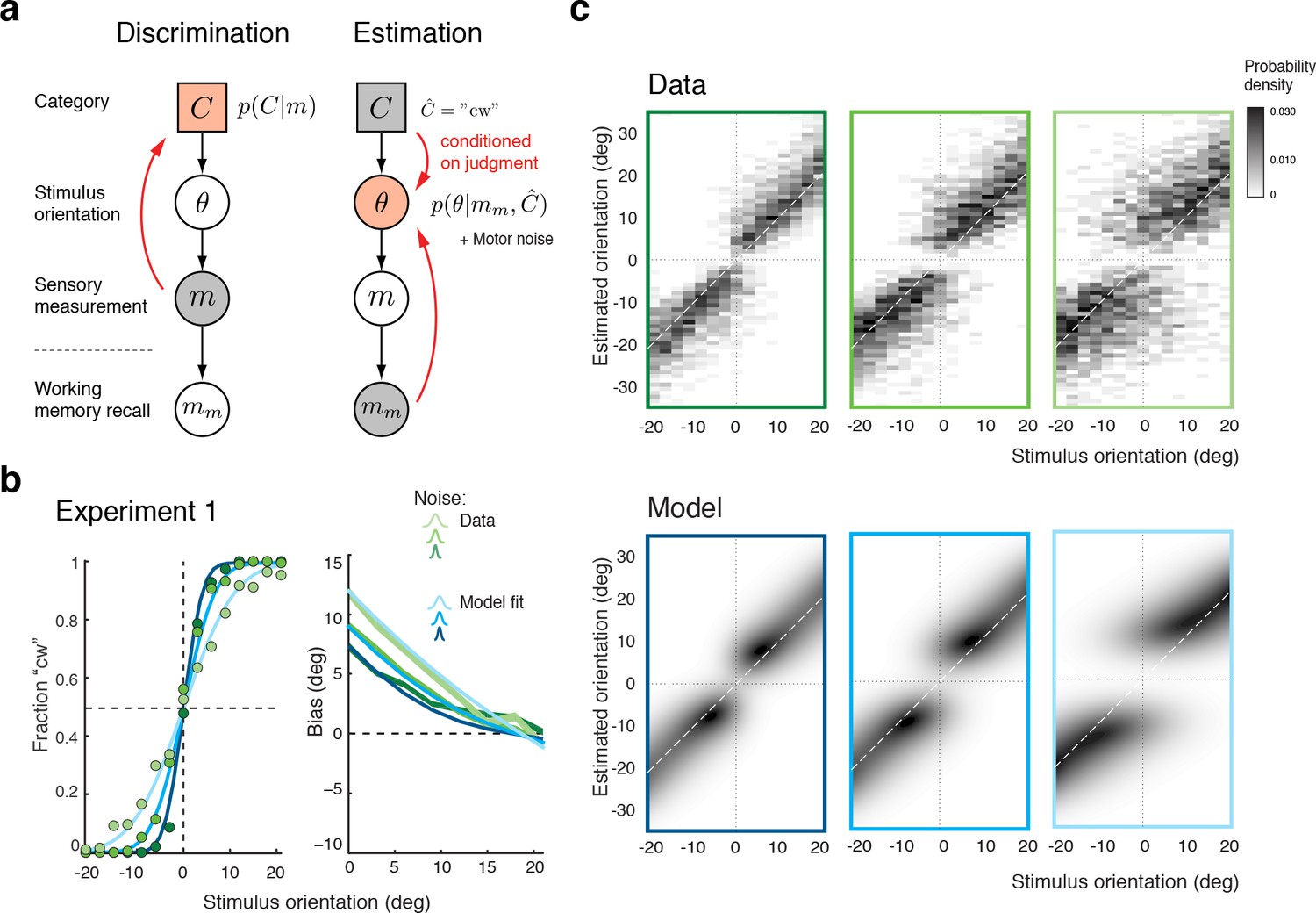
The self-consistent Bayesian observer model.
(a) Directed graph representing the generative hierarchical model: Sensory measurement is a noisy sample of stimulus orientation . Every belongs to one of two categories . Given an observed , the self-consistent model first performs inference over (discrimination task), and then infers the value of conditioned on the preceding discrimination judgment (e.g., ) (estimation task). Inference for the estimation task is assumed to be based on a noisy memory recall of the sensory measurement . Conditioning on the categorical choice sets the posterior to zero for all values of that do not agree with the choice. This shifts the posterior probability mass away from the discrimination boundary and results in the repulsive post-decision biases for any loss function that more strongly penalizes large errors than small ones. Because subjects were instructed to provide estimates as accurate as possible we assumed a loss function that minimizes mean squared-error ( loss). (b) We jointly fit the observer model to all discrimination-estimation data pairs of the combined data across all subjects in Experiment 1 (combined subject). (c) The model not only predicts the mean estimation bias (as shown in (b)) but also the entire distributions of estimates, including those trials where discrimination judgments were incorrect. Data and model show the characteristic bimodal pattern for orientation estimates. Each column corresponds to one of the three stimulus noise conditions.
Figure 3—figure supplement 1
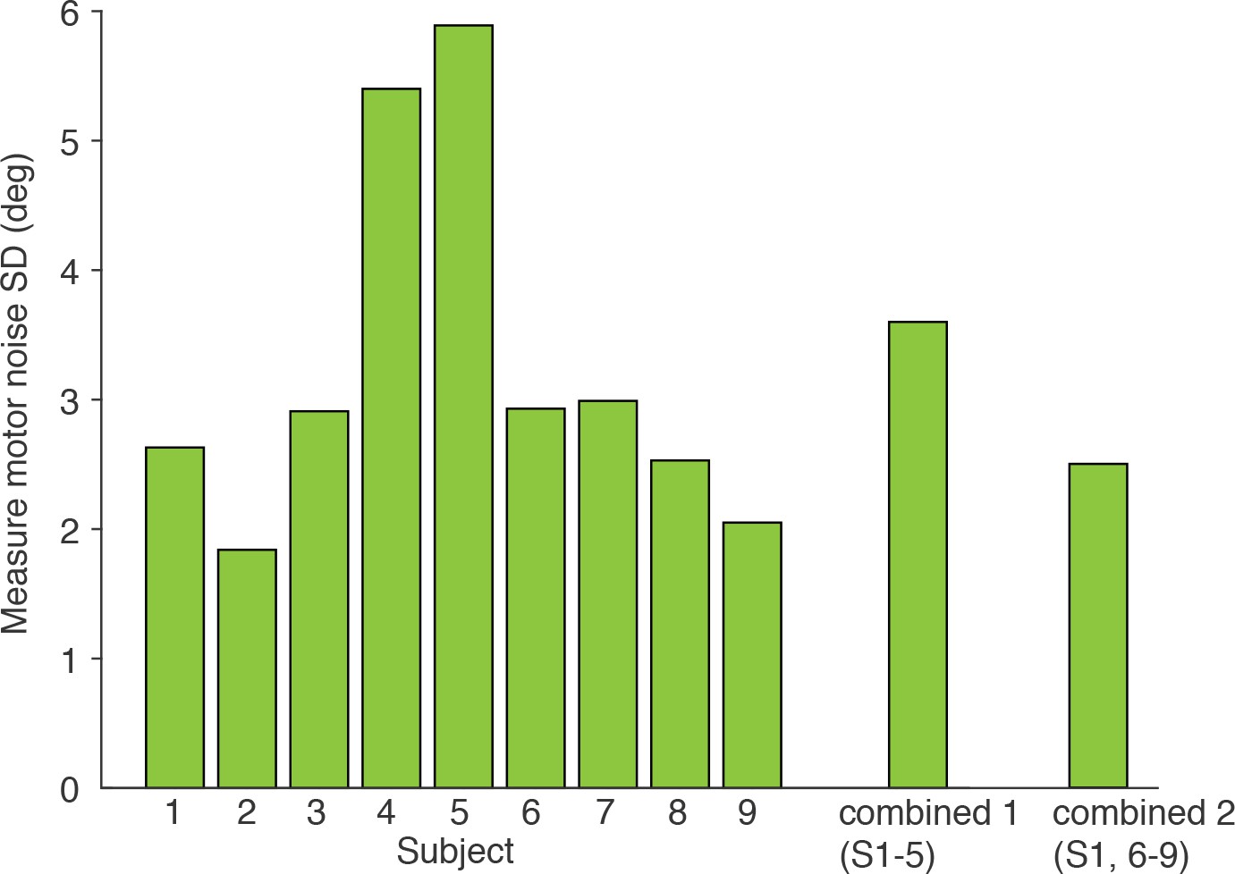
Measured motor noise of individual subjects.
Shown are the extracted values of the standard deviation in subjects’ estimates in the control experiment (see Materials and methods). These individual values were used in modeling the data from Experiment 1–3, assuming that motor noise was Gaussian distributed.
Figure 3—figure supplement 2
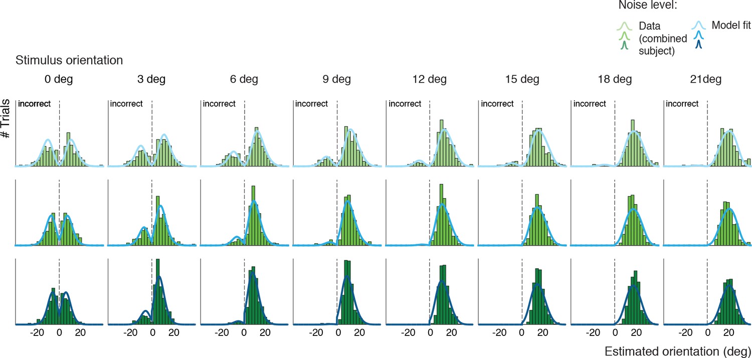
Histogram plots of the orientation estimates together with the model fit for Experiment 1 (combined subject).
Each row is for one of the three stimulus noise conditions.
Figure 4 with 1 supplement
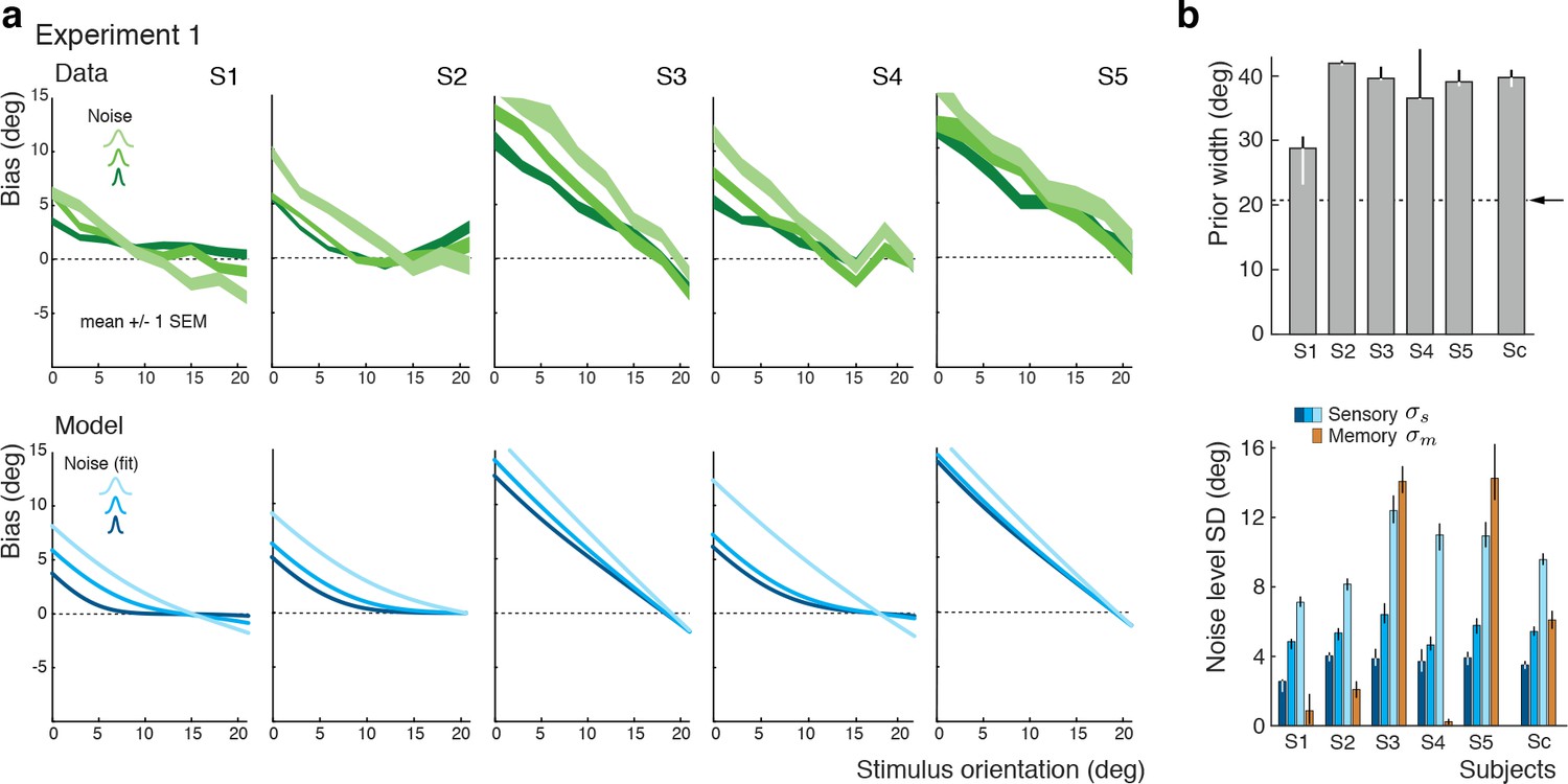
Experiment 1: Data and model fits for individual subjects.
(a) Individual subjects (S1 non-naïve) showed substantial variations in their bias patterns (green curves). These variations are well explained by individual differences in the fit parameter values of the self-consistent model (blue curves). For example, the width of the prior directly determines the location where the bias curves intersect with the x-axis. (b) Fit prior widths and noise levels for the five individual subjects plus the combined subject (Sc). Subjects’ prior widths suggest that they consistently overestimated the actual stimulus range in the experiment (± 21 degrees; arrow). For all subjects, fit sensory noise was comparable and monotonically dependent on the actual stimulus noise. Memory noise was mostly small as expected, yet dominated for subjects S3 and S5. These two subjects performed poorly in the estimation task, suggesting that they were not trying to provide an accurate orientation estimate but simply pointed the cursor to roughly the middle of the stimulus range on the side of the discrimination boundary they picked in the discrimination task. The resulting bias curves are basically independent of the stimulus noise and have a slope of approximately −1. The model captured this behavior by assuming that the sensory information was ‘washed out’ with a large amount of memory noise. The full model also contained a motor noise component that was determined for each subject in a separate control experiment. All errorbars represent the 95% confidence interval computed over 100 bootstrapped sample sets of the data. See Materials and methods for details.
Figure 4—figure supplement 1
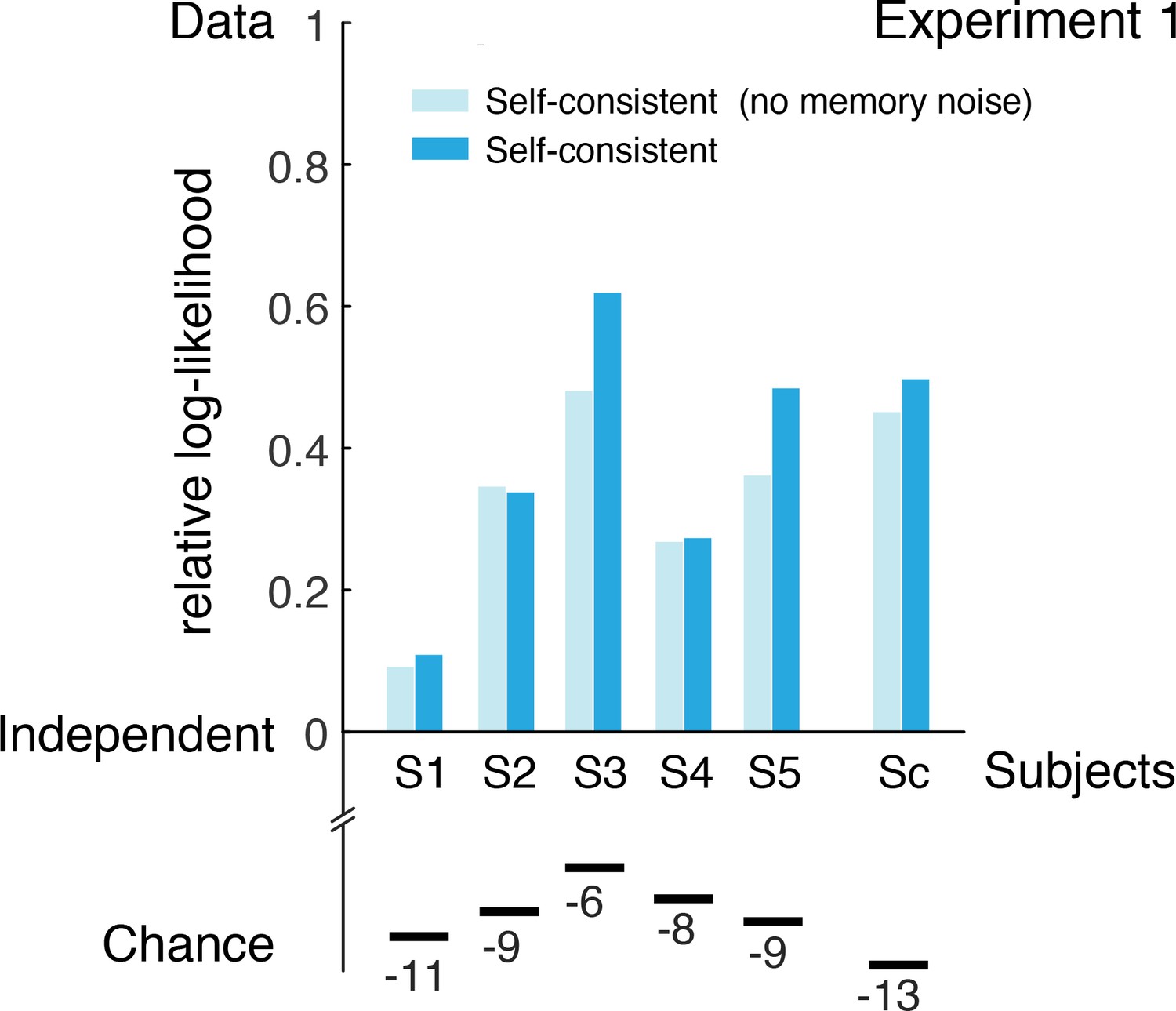
Goodness-of-fits for Experiment 1.
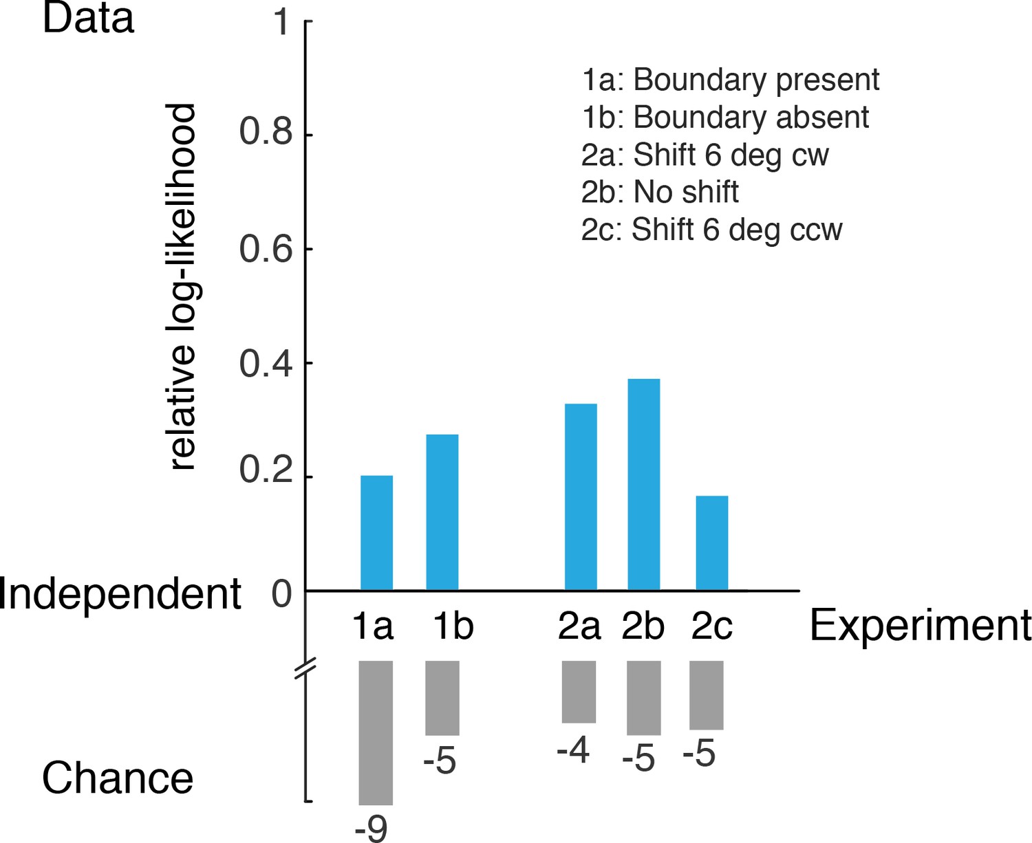
Log-likelihood values of the fit self-consistent observer model for every subject (as well as the combined subject Sc), relative to the range defined by the likelihoods of the independent Bayesian observer and a hypothetical, omniscient model (’Data’). The latter can be thought of as the data explaining itself, that is, a model 'defined’ by the empirical probabilities of the data. The log-likelihoods of a random observer (’Chance’) are also given as additional reference. This observer can be thought of as 'being blind’, thus providing random answers in both the discrimination task and the estimation task (sampling from a uniform distribution). The self-consistent observer model is consistently outperforming the independent Bayesian model in explaining the data. Note, the self-consistent and the independent observer model have exactly the same model parameters. Also, a version of the self-consistent observer model that does not include noise in the memory recall of the sensory signal (Stocker and Simoncelli, 2007) generally does not fit the data as well.
Figure 5 with 1 supplement

Effect of the stimulus prior.
(a) Experiment 2 was identical to Experiment 1 except that at the beginning of each trial, subjects were shown the total range within which the stimulus orientation would occur in the trial (gray arc, subtending 21 degrees). (b) We hypothesize that reminding subjects of the exact stimulus range at the beginning of each trial helps them to form a more accurate (and more narrow) representation of their stimulus prior. If subjects’ orientation estimates were indeed the result of the conditioned Bayesian inference as assumed by the self-consistent observer model, then the bias curves should shift towards the discrimination boundary. The data support this prediction: Subjects’ bias curves (combined subject, see Figure 7 for individual subjects) are shifted towards the discrimination boundary compared to Exp. 1. (c) As with Exp.1, the fit self-consistent model provides an accurate description of the distribution pattern of subjects’ orientation estimates.
Figure 5—figure supplement 1
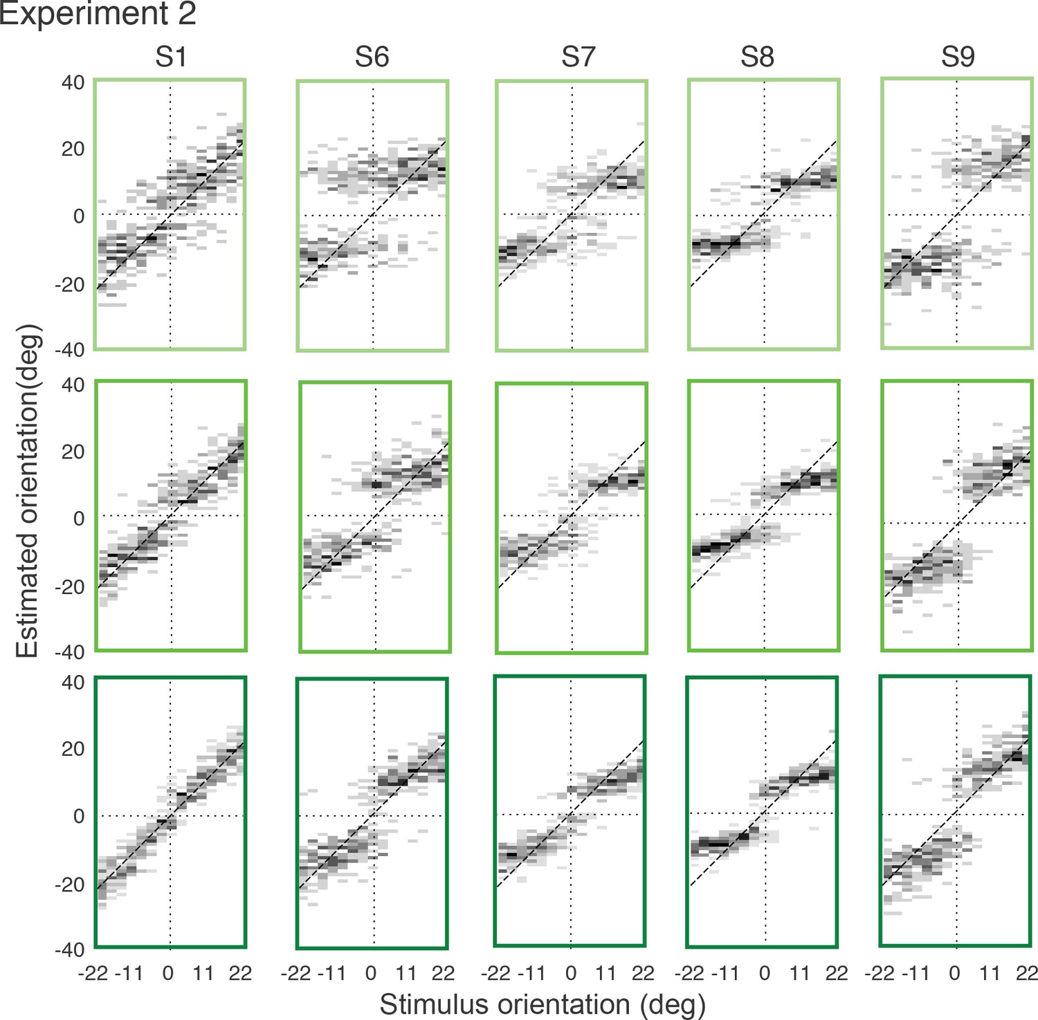
Full distributions of individual subjects’ estimates in Experiment 2.
Each row corresponds to one of the three stimulus noise conditions (top-bottom: highest-lowest; color-code as in main text).
Figure 6 with 1 supplement
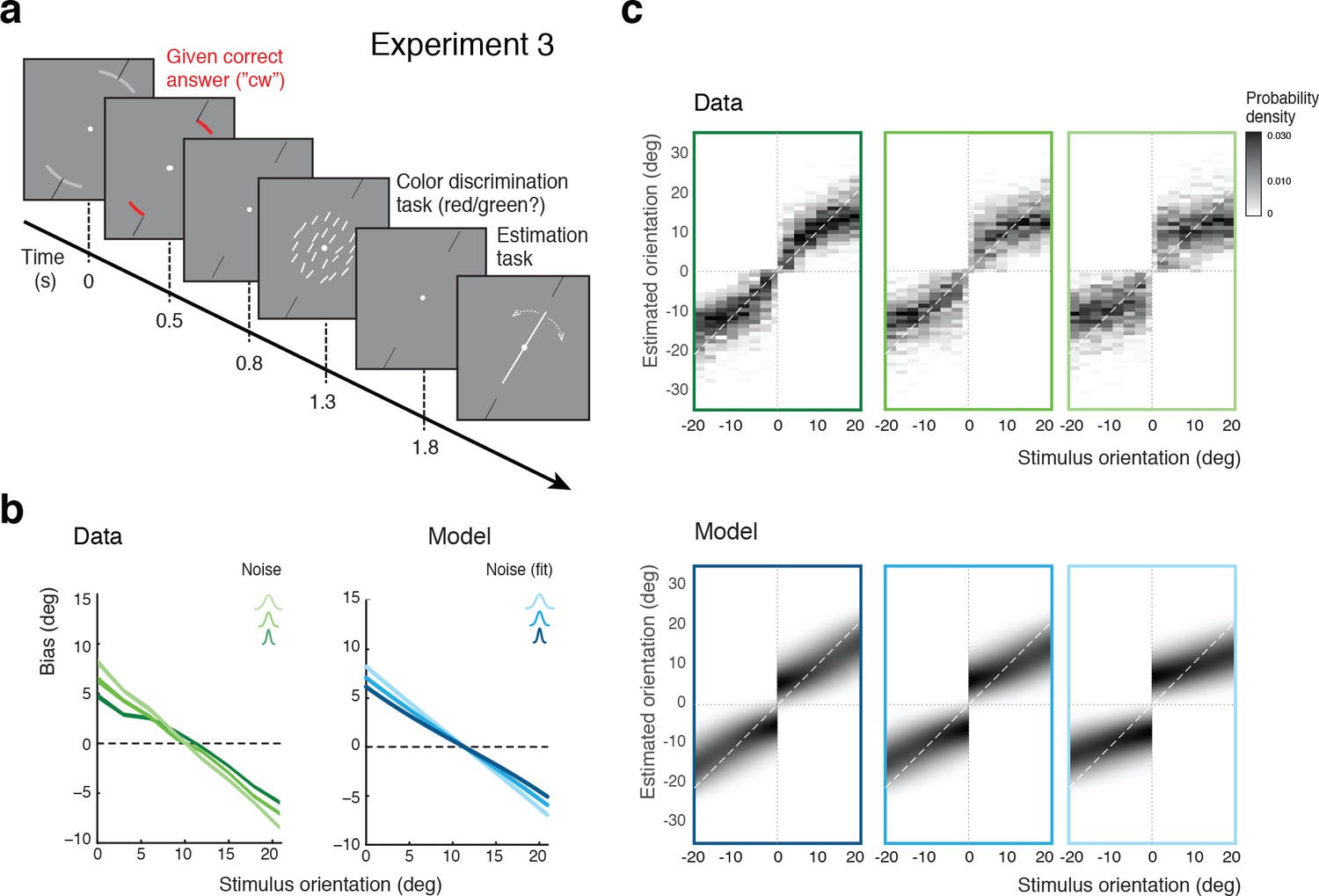
Self-made vs. given category assignment.
(a) Experiment 3: Instead of performing the discrimination judgment themselves, subjects were provided with a cue indicating the correct category assignment right before the stimulus was presented. Then, after stimulus presentation, subjects first performed an unrelated color discrimination task in place of the orientation discrimination task (they needed to remember the randomly assigned color (red/green) of the cue indicating the correct category) before indicating their perceived stimulus orientation. (b) According to our model we should see similar estimation biases in Exps. 2 and 3, which is indeed what we found. (c) Again, the fit model well accounts for the overall distribution of orientation estimates (combined subject; see Figure 6—figure supplement 1 for distributions for individual subjects)). Because the discrimination judgment was given and always correct independent of the noise in the sensory measurement , estimates only occurred in the ‘correct’ quadrants. For the same reason the model also predicts slightly smaller bias magnitudes (compared to Exp.2), which is also matched by the data (see also Figure 7b).
Figure 6—figure supplement 1
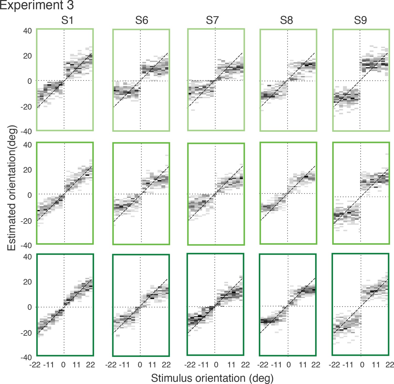
Full distributions of individual subjects’ estimates in Experiment 3.
Each row corresponds to one of the three stimulus noise conditions (top-bottom: highest-lowest; color-code as in main text).
Figure 7 with 1 supplement
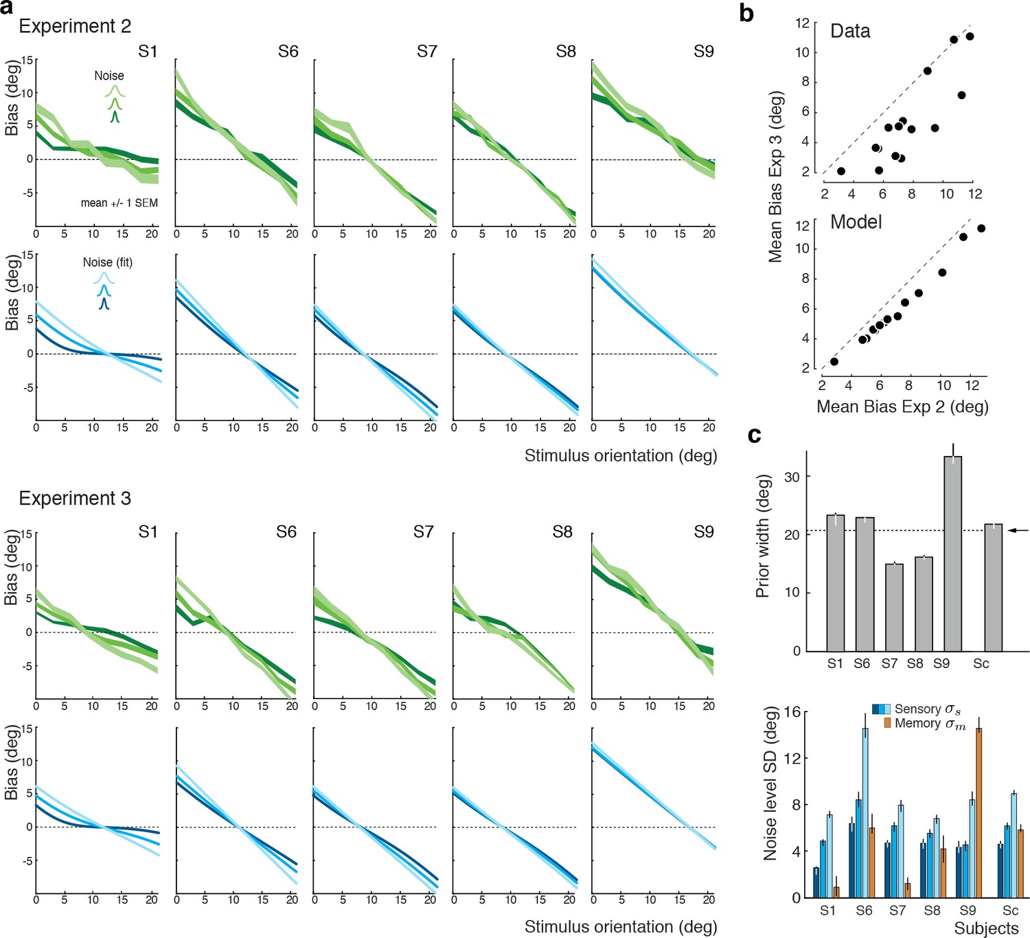
Experiments 2 and 3: Joint fit to data for individual subjects.
(a) Five subjects (S1, S6-9) participated both in Exp. 2 and 3. We performed a joint model fit to the data from both experiments for every subject. Each column shows data (green curves) and fit (blue curves) for a particular subject. As in Exp. 1, the bias pattern across subjects shows substantial variability yet is strikingly similar between the two experiments. (b) Comparing the mean biases observed in Exps. 2 and 3 reveals that biases in Exp. 3 are slightly smaller for stimulus orientations close to the boundary. This effect is predicted by the model. (c) Fit prior widths and noise levels for individual subjects and the combined subject. Subjects’ priors were closer to the experimental distribution than in Exp. 1 because in Exps. 2 and 3 subjects were reminded about the stimulus range at the beginning of each trial. Noise levels were comparable to those in Exp. 1 (for S1 we jointly fit data from all three experiments). Errorbars indicated the 95% confidence interval over 100 bootstrapped samples of the data. See Figure 7—figure supplement 1 for a goodness-of-fit analysis.
Figure 7—figure supplement 1
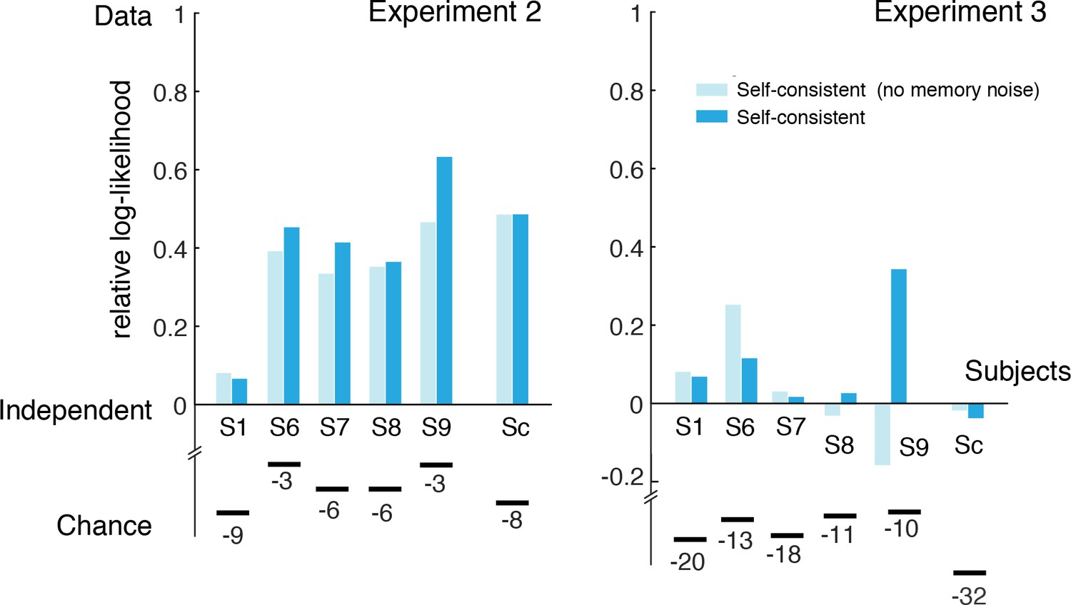
Goodness-of-fits for Experiments 2 and 3.
Relative log-likelihood values of the fit self-consistent observer model for every subject (as well as the combined subject Sc). Relative scale is defined as described for Figure 4—figure supplement 1. The self-consistent observer model is consistently outperforming the independent Bayesian model in explaining data from Experiment 2. For Experiment 3 both models are formally identical; the marginal differences in likelihood are simply because their fit parameter values slightly differ due to the joint fit to data from both Experiments 2 and 3 (subject S1; joint fit to all three experiments). Note, the self-consistent and the independent observer model have exactly the same model parameters. Also, a model that does not include noise in the memory recall of the sensory signal generally does not fit the data as well as the full self-consistent observer model.
Figure 8
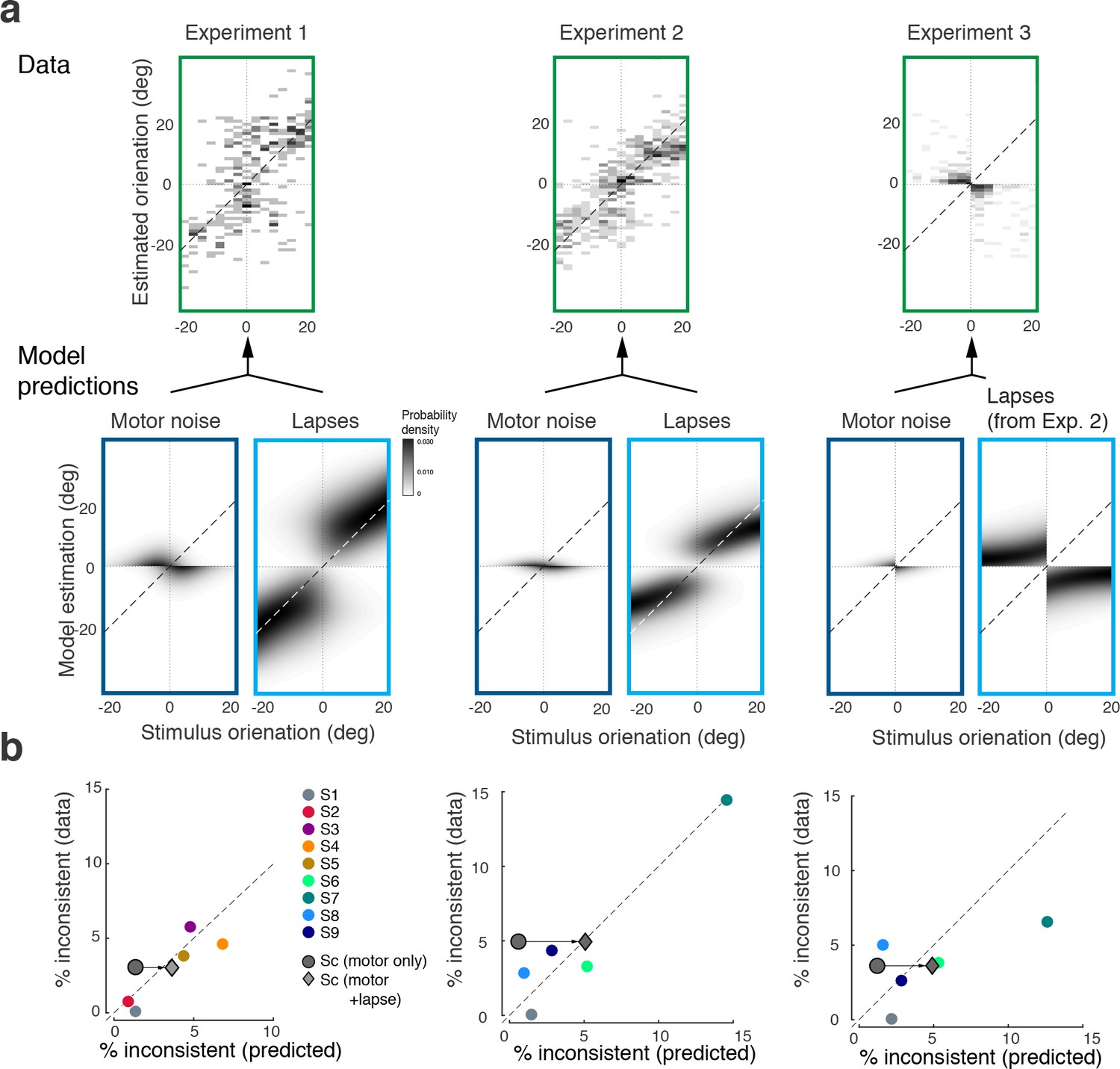
Inconsistent trials are due to lapses and motor noise.
(a) Distribution of estimates for the small fraction of inconsistent trials (4% of the data) in each experiment (across all subjects and stimulus noise conditions). The estimation patterns can be explained as a weighted superposition of two sources of erroneous, non-perceptual behavior: lapses and motor noise. The self-consistent model well predicts the estimation patterns. All predictions are based on parameter values taken from the model fit to the consistent trial data (see Materials and methods). Lapse rates were extracted from the psychometric functions of the discrimination judgment for the total data. Motor noise was measured in a control experiment (see Materials and methods, Figure 3—figure supplement 1). (b) Quantitative predictions for each subject’s total fraction of inconsistent trials are compared to the measured fractions. Predictions for the combined subjects suggest that inconsistent trials are mainly due to lapses.
Figure 9
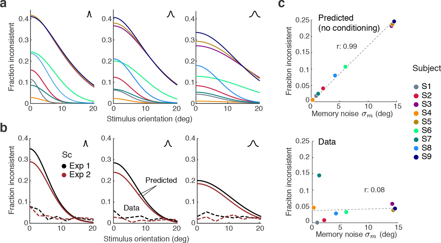
Maintaining self-consistency in the face of working memory noise.
(a) Shown are the predicted fractions of inconsistent trials if orientation estimates are not conditioned on the preceding judgment. These are trials for which the sensory signal and its memory recall are on different sides of the discrimination boundary. Using the fit model parameters from Exps. 1 and 2, each curve represents the fraction of inconsistent trials as a function of stimulus orientation for every subject (color code on the right). Each panel is for one of the three stimulus noise conditions. These large fractions are predicted for any non-trivial model whose discrimination judgment is based on and the estimate on but does not condition the estimation process on the preceding discrimination judgment. For simplicity, we did not include lapses and motor error for this analysis, and thus these predictions reflect the direct consistency benefit of conditioning the estimate on the preceding discrimination judgment. (b) The actual fractions of inconsistent trials are much lower and relatively independent of stimulus orientation as they are mostly due to lapses (see Figure 8b); shown is the combined subject. (c) The benefit of self-consistent inference is substantial for larger memory noise; predicted fractions are almost perfectly correlated with the fit memory noise of individual subjects. In comparison, the actual fractions of inconsistent trials are uncorrelated with memory noise levels, in line with our previous analysis showing that they are mainly due to lapses and motor noise.
Figure 10 with 3 supplements
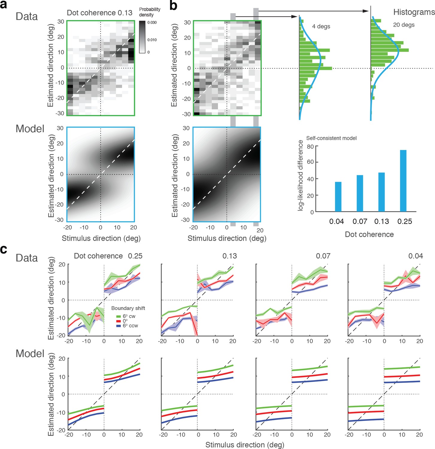
Model fits for experimental data by Zamboni et al., (2016).
(a) Experiment 1a: Exact replication of the original experiment (Jazayeri and Movshon, 2007). Exemplarily shown is the estimation data (combined subject) at one stimulus coherence level (0.13) together with our model fit. (b) Experiment 1b was identical except that the boundary was not shown during the estimation task. Estimate distributions are no longer bimodal yet the self-consistent observer, relying on a noisy memory of the boundary orientation, consistently better fit the data than the independent observer model (log-likelihood difference). (c) Experiment 2 introduced a shift in the boundary orientation right before the estimation task, which subjects were not aware of (six degrees). Subjects’ estimates were shifted accordingly (combined subject). The self-consistent model can account for the shift if we assume that the conditional prior is applied to the shifted boundary orientation. See Figure 10—figure supplements 1–3 for distributions, fits, and goodness-of-fits for all conditions.
Figure 10—figure supplement 1
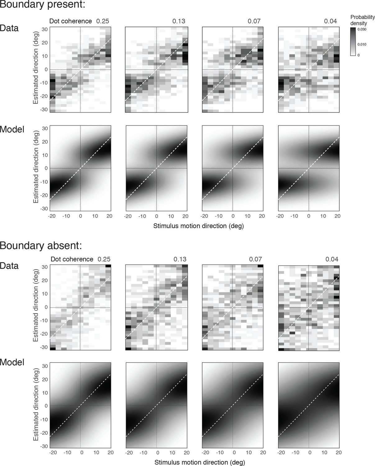
Zamboni et al., (2016) data (Experiment 1, combined subject) and fit with the self-consistent observer model.
https://doi.org/10.7554/eLife.33334.019
Figure 10—figure supplement 2
Relative log-likelihoods of model fits for Zamboni et al., (2016) data.
Relative log-likelihood values of the self-consistent observer model fit to the combined subject data for each experiment. Relative scale is defined as described for Figure 4—figure supplement 1.
Figure 10—figure supplement 3
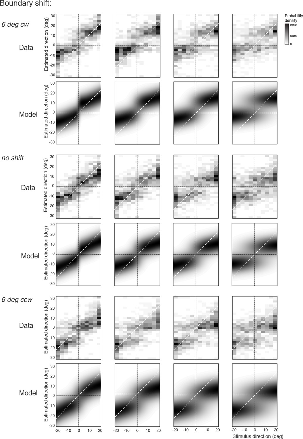
Zamboni et al., (2016) data (Experiment 2, combined subject) and fit with the self-consistent observer model.
https://doi.org/10.7554/eLife.33334.021Additional files
-
Source data 1
Data for Experiment 1.
- https://doi.org/10.7554/eLife.33334.022
-
Source data 2
Data for Experiment 2.
- https://doi.org/10.7554/eLife.33334.023
-
Source data 3
Data for Experiment 3.
- https://doi.org/10.7554/eLife.33334.024
-
Transparent reporting form
- https://doi.org/10.7554/eLife.33334.025
Download links
A two-part list of links to download the article, or parts of the article, in various formats.
Downloads (link to download the article as PDF)
Open citations (links to open the citations from this article in various online reference manager services)
Cite this article (links to download the citations from this article in formats compatible with various reference manager tools)
Post-decision biases reveal a self-consistency principle in perceptual inference
eLife 7:e33334.
https://doi.org/10.7554/eLife.33334


