Figures and data in Current CRISPR gene drive systems are likely to be highly invasive in wild populations

Version of Record: June 19, 2018

Download
A two-part list of links to download the article, or parts of the article, in various formats.
Downloads (link to download the article as PDF)
- Article PDF
Open citations (links to open the citations from this article in various online reference manager services)
- Mendeley
Cite this article (links to download the citations from this article in formats compatible with various reference manager tools)
Charleston Noble

Ben Adlam

George M Church

Kevin M Esvelt

Martin A Nowak

(2018)
Current CRISPR gene drive systems are likely to be highly invasive in wild populations

eLife 7:e33423.

https://doi.org/10.7554/eLife.33423
- Download BibTeX
- Download .RIS
Cite
Share
CommentOpen annotations (there are currently 0 annotations on this page).

Figures
Tables
Additional files

11 figures, 3 tables and 1 additional file

Figures

Figure 1

Download asset Open asset

Existing alteration-type CRISPR gene drive systems should invade well-mixed wild populations.

(A) Typical construction and function of alteration-type CRISPR gene drive systems. A drive construct (D), including a CRISPR nuclease, guide RNA (gRNA), and ‘cargo’ sequence, induces cutting at a …
https://doi.org/10.7554/eLife.33423.003

Figure 2

Download asset Open asset

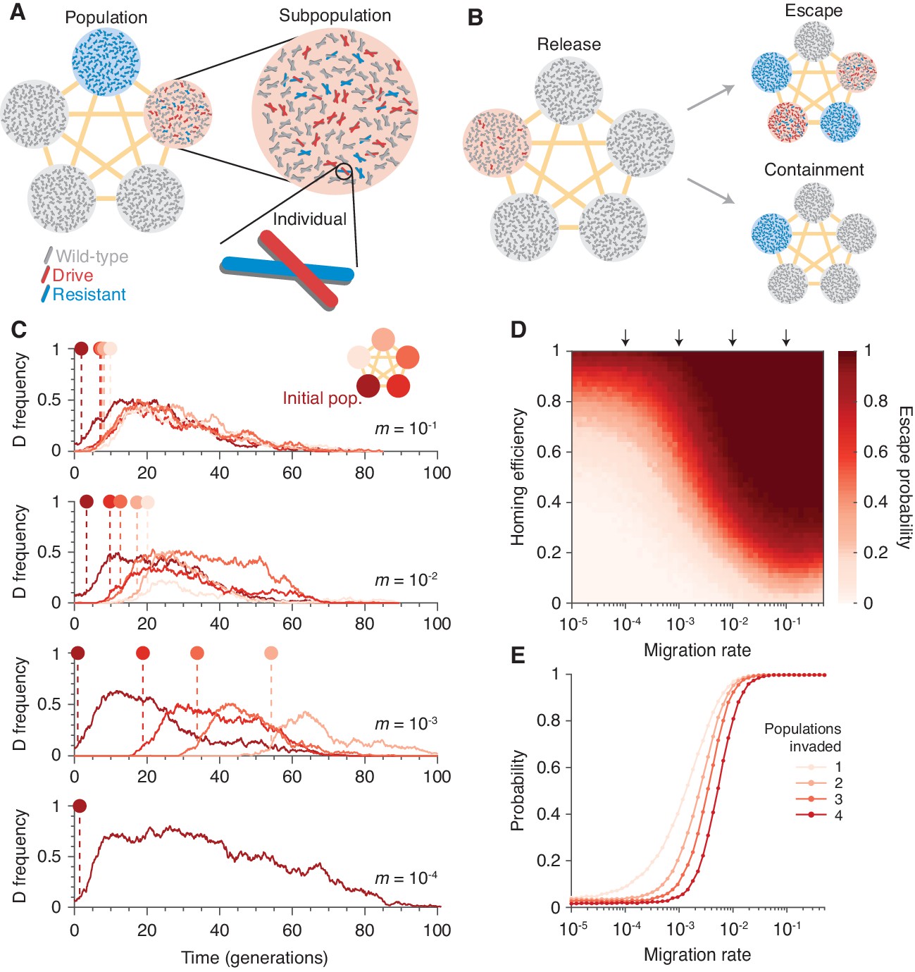
Existing CRISPR gene drive systems should invade linked subpopulations connected by gene flow.

(A) Diagram of well-mixed subpopulations (circles) linked by gene flow (edges). Individuals represented by chromosomes with wild-type (gray), drive (red), or resistant (blue) haplotypes. (B) Few …
https://doi.org/10.7554/eLife.33423.004

Figure 3

Download asset Open asset

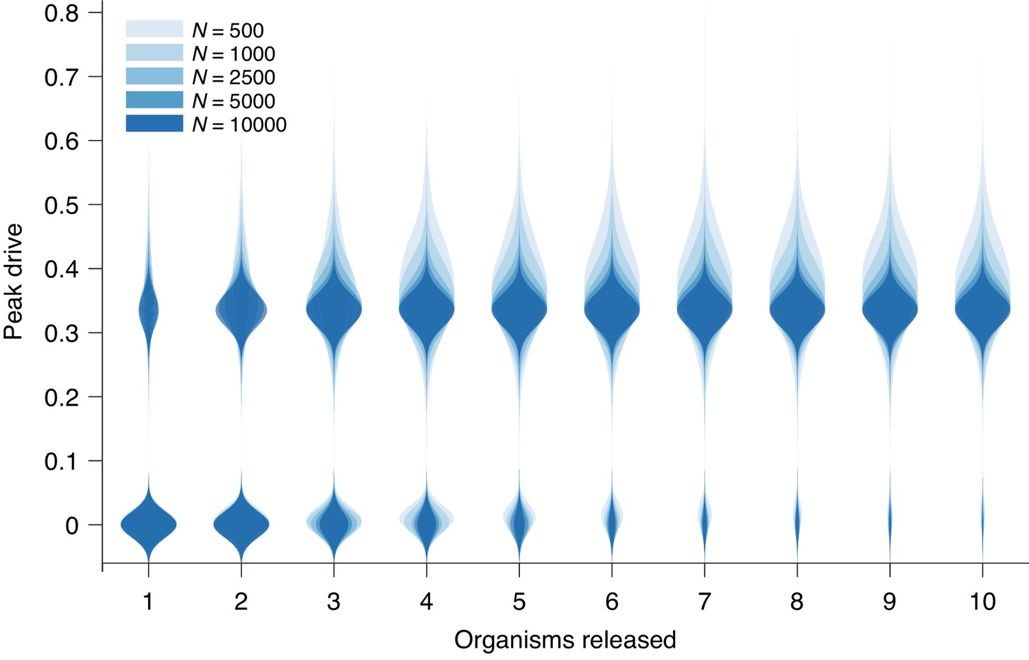
Peak drive distributions for variable release and population sizes.

Parameters are chosen to correspond to Figure 1E: $P = 0.5$ , $f = 0.9$ and neutral resistance. Population sizes are, from light to dark, $N = 500, 1000, 2500, 5000, 10000$ . Note that $N = 500$ corresponds exactly to Figure 1E. Each distribution …
https://doi.org/10.7554/eLife.33423.005

Figure 4

Download asset Open asset

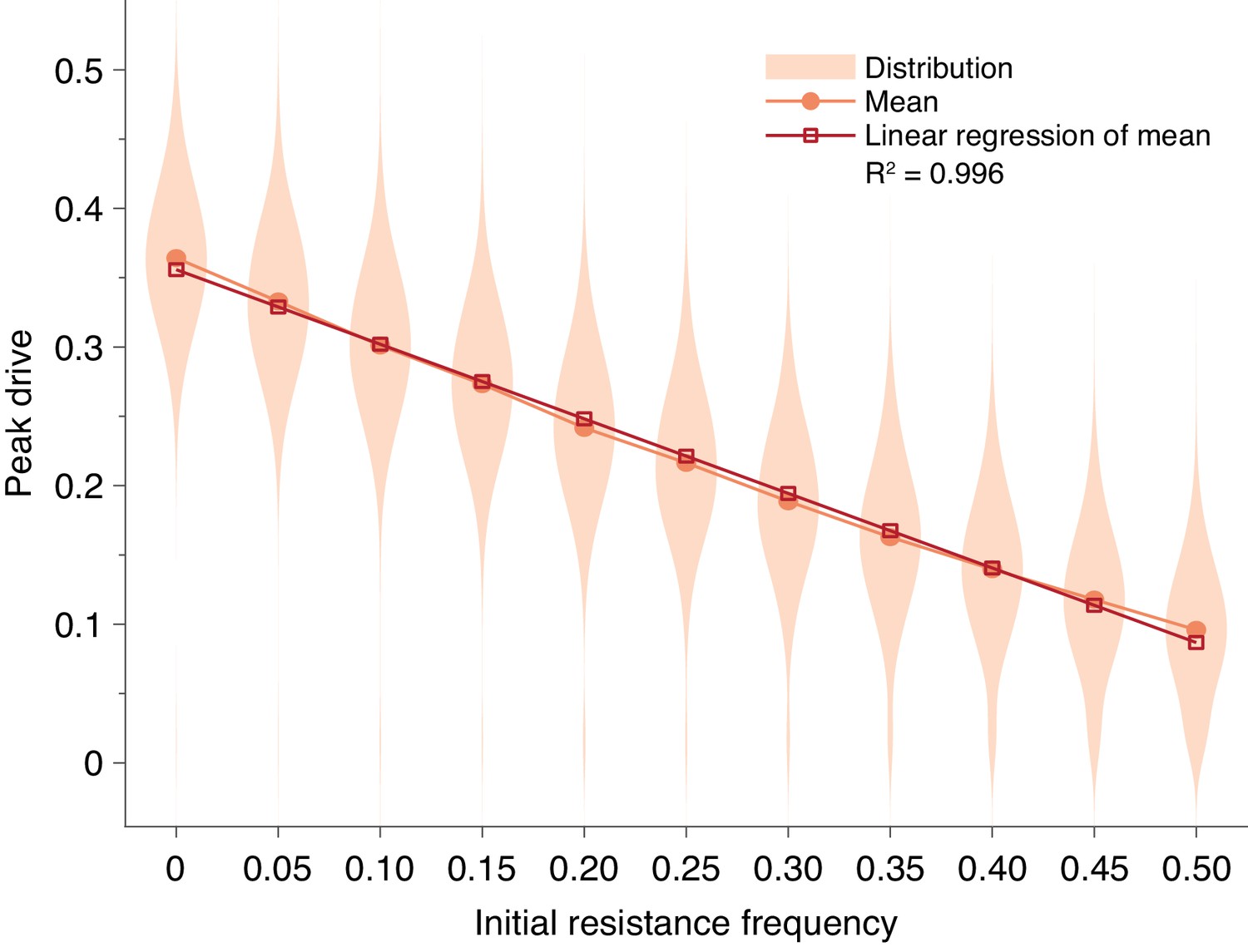
Pre-existing drive-resistant allele frequency linearly decreases peak drive.

Distributions (violin plots), means (orange, circles) and linear regression of the mean values (red, squares). Parameters are chosen to correspond to Figure 1E: $P = 0.5$ , $f = 0.9$ , neutral resistance, $N = 500$ . Each …
https://doi.org/10.7554/eLife.33423.006

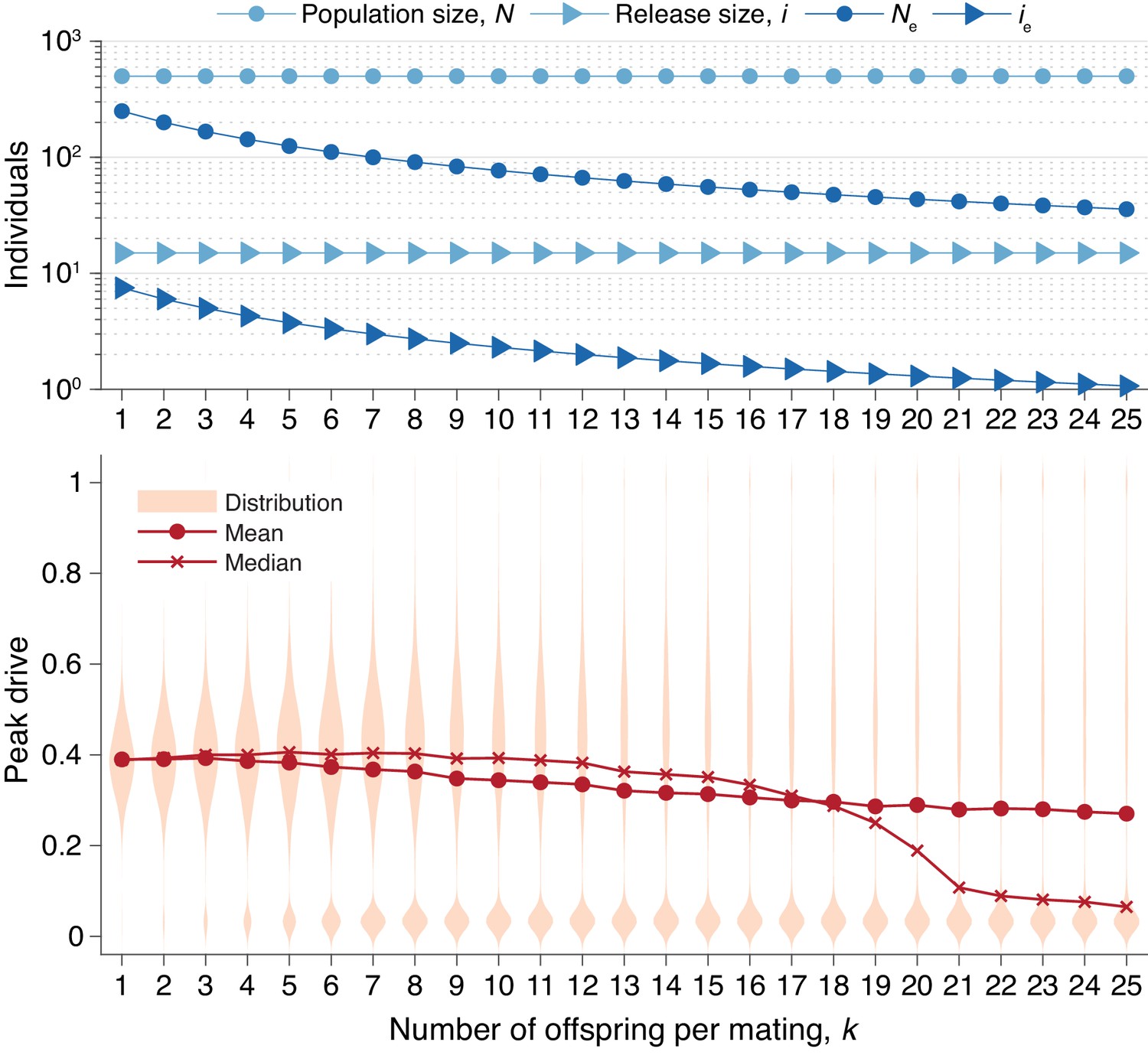
Figure 5

Download asset Open asset

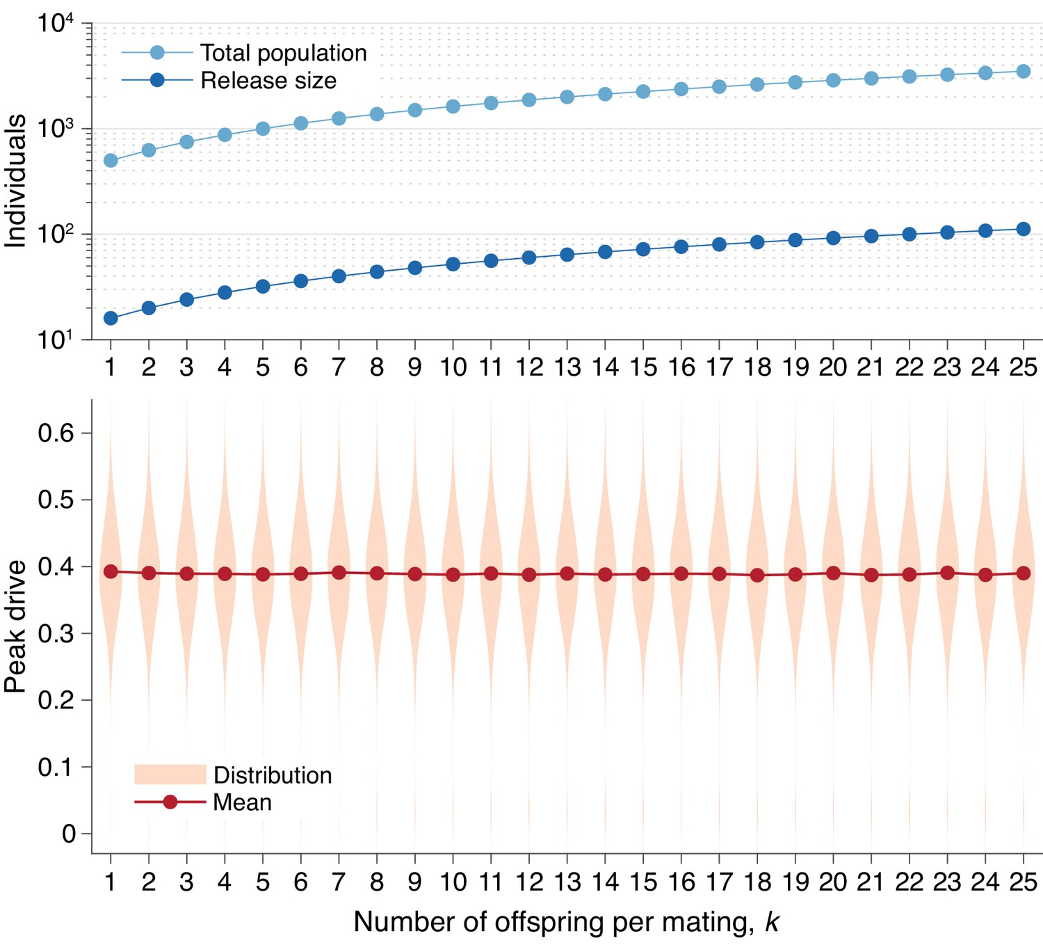
Peak drive distributions for varying numbers of offspring per mating with effective population and release sizes held constant.

(top) Population and release sizes used in the simulations below. For the case $k = 1$ , we use our usual population size of $N = 500$ with an initial release of $i = 16$ drive homozygotes. According to Equation (5), …
https://doi.org/10.7554/eLife.33423.007

Figure 6

Download asset Open asset

Peak drive distributions for varying numbers of offspring per mating with census population and actual release sizes held constant.

(top) Population and release sizes used in the simulations below. Actual population size, $N$ (light blue, circles) and actual release size, $i$ (light blue, triangles). Note that $N = 500$ and $i = 15$ are …
https://doi.org/10.7554/eLife.33423.008

Figure 7

Download asset Open asset

Mean peak drive for varying homing efficiency, $P$ , and drive-individual fitness values, $f$ (i.e., individuals with genotypes WD, DD, and DR), assuming that fitness affects birth rate (left) or death rate (right).

The left panel corresponds to our standard model, shown in Figure 1C, while the right panel represents a modification: parents are chosen uniformly, and individuals die with probability proportional …
https://doi.org/10.7554/eLife.33423.009

Figure 8

Download asset Open asset

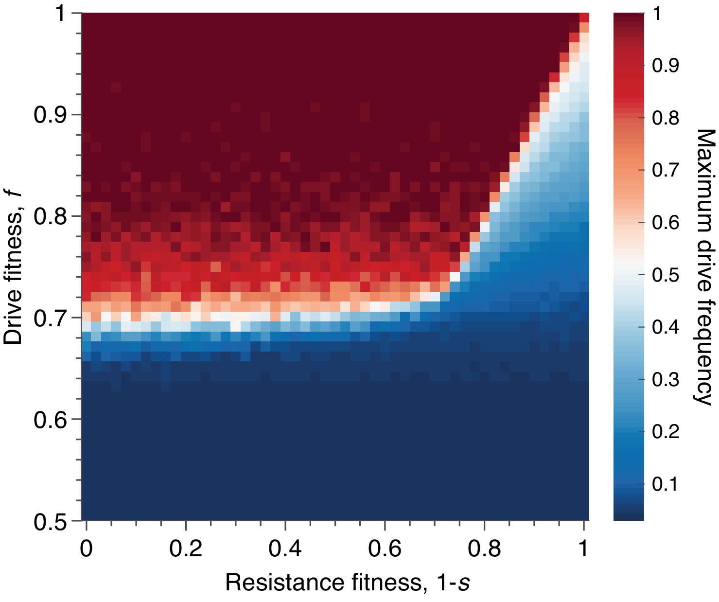
Mean peak drive for varying drive-individual fitness values, $f$ , and resistant-individual (RR) fitness values, $1 - s$ , where $s$ is the cost associated with resistance.

Each point in the grid ( $51 \times 51$ ) depicts an average of 100 simulations. Parameters used include homing efficiency $P = 0.5$ , population size of 500, with an initial release of 15 drive homozygotes to ensure …
https://doi.org/10.7554/eLife.33423.010

Figure 9

Download asset Open asset

Peak drive distributions and means for varying selfing rates in our partial selfing model.

(top) Effective drive, $P = 0.9$ . (middle) conservative drive, $P = 0.5$ , and (bottom) constitutive drive, $P = 0.15$ . Each distribution comprises $1000$ simulations. Parameters used include a population size of 500 with an …
https://doi.org/10.7554/eLife.33423.011

Figure 10

Download asset Open asset

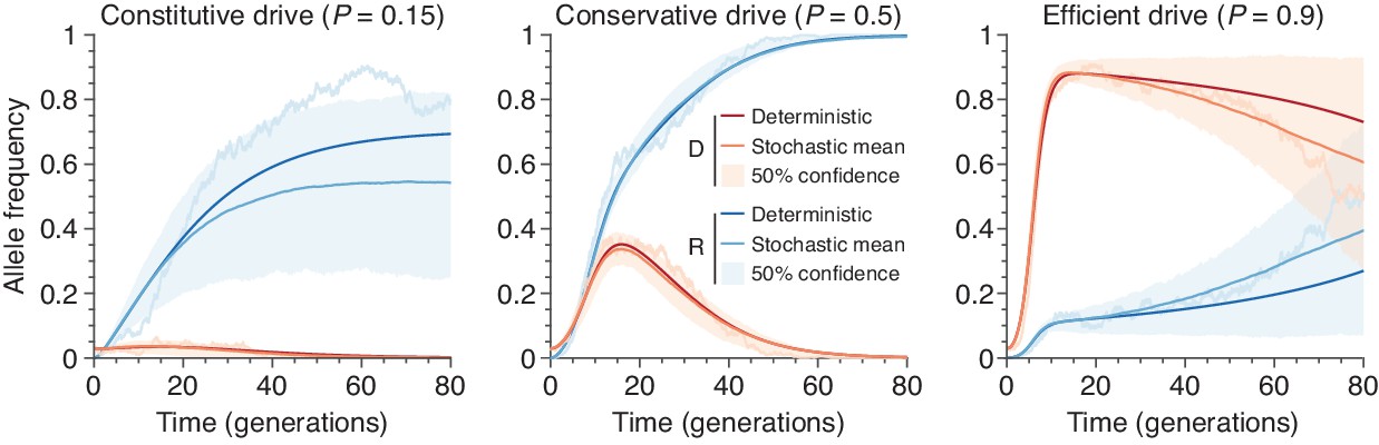
Finite-population simulations of 15 drive individuals released into a wild population of size 500, assuming low ( $P = 0.5$ ) or high ( $P = 0.9$ ) homing efficiencies, as well as a low-efficiency, constitutively active system ( $P = 0.15$ ).

Deterministic results (dark lines) and means of $10^{3}$ simulations (medium lines), individual sample simulations (light lines), and 50% confidence intervals (shaded). Drive frequencies red and …
https://doi.org/10.7554/eLife.33423.012

Figure 11

Download asset Open asset

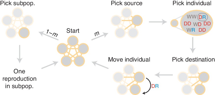
Diagram of simulation scheme.

In each time step, a migration occurs with probability $m$ , or a mating happens with probability $1 - m$ . If a migration occurs, a source population is chosen randomly proportional to its size; an …
https://doi.org/10.7554/eLife.33423.013

Tables

Appendix 1—table 1

Empirical homing efficiencies for all CRISPR gene drive systems published to date.

Details can be found in the Appendix.

https://doi.org/10.7554/eLife.33423.016

Organism	Ref.	System name	Efficiency
Yeast	(DiCarlo et al., 2015)	ade2::sgRNA	$> 99 %$
		ade2::sgRNA + URA3	$100 %$
		sgRNA + ABD1	$100 %$
		cas9 + sgRNA	$> 99 %$
		ADE2 + sgRNA + cas9	$> 99 %$
Fruit flies	(Gantz and Bier, 2015)	$γ$ -MCR	$97 %$
	(Champer et al., 2017)	nanos	$62 %$
		vasa	$52 %$
		additional nanos	40–62%
		additional vasa	37–53%
Mosquitoes	(Gantz et al., 2015)	AsMCRkh2 (male)	$98 %$
		AsMCRkh2 (female)	$14 %$
	(Hammond et al., 2016)	AGAP011377	$83 %$
		AGAP005958	$95 %$
		AGAP007280	$99 %$

Appendix 1—table 2

Gantz et al., An. stephensi transgenic male lines.

(left) Phenotypes of G $_{3}$ progeny. (right) Phenotypes of G $_{4}$ progeny.

https://doi.org/10.7554/eLife.33423.017

G $_{3}$ crosses	$D$	$T$	Reference
$10.1$ G $_{2}$ $\times$ WT, larval	$829$	$832$	Table S3
$10.2$ G $_{2}$ $\times$ WT, larval	$3060$	$3085$	Table S4
$10.1$ G $_{2}$ $\times$ WT, adult	$833$	$836$	Table S5
$10.2$ G $_{2}$ $\times$ WT, adult	$1258$	$1274$	Table S6
Total	$5980$	$6027$	—
G $_{4}$ crosses	$D$	$T$	Reference
Cross 6, larval	$949$	$955$	Table S7
Cross 8, larval	$609$	$628$	Table S8
Cross 6, adult	$882$	$888$	Table S10
Cross 8, adult	$565$	$583$	Table S11
Total	$3005$	$3054$	—

Appendix 1—table 3

Gantz et al., An. stephensi transgenic male lines.

(left) Phenotypes of G $_{4}$ larvae. (right) Phenotypes of G $_{4}$ adults.

https://doi.org/10.7554/eLife.33423.018

G $_{4}$ larvae	$D$	$T$	Reference
Cross $1$	$28$	$48$	Table S7
Cross 2	$332$	$635$	Table S7
Cross 3	$204$	$324$	Table S8
Cross 4	$372$	$632$	Table S8
Total	$936$	$1639$	—
G $_{4}$ adults	$D$	$T$	Reference
Cross 1	$19$	$35$	Table S10
Cross 2	$306$	$554$	Table S10
Cross 3	$169$	$272$	Table S11
Cross 4	$1430$	$2500$	Table S11
Total	$1924$	$3361$	—

Additional files

Transparent reporting form: https://doi.org/10.7554/eLife.33423.014
Download elife-33423-transrepform-v1.pdf

Downloads (link to download the article as PDF)

Open citations (links to open the citations from this article in various online reference manager services)

Cite this article (links to download the citations from this article in formats compatible with various reference manager tools)

Figures

Existing alteration-type CRISPR gene drive systems should invade well-mixed wild populations.

Existing CRISPR gene drive systems should invade linked subpopulations connected by gene flow.

Peak drive distributions for variable release and population sizes.

Pre-existing drive-resistant allele frequency linearly decreases peak drive.

Peak drive distributions for varying numbers of offspring per mating with effective population and release sizes held constant.

Peak drive distributions for varying numbers of offspring per mating with census population and actual release sizes held constant.

Mean peak drive for varying homing efficiency, $P$ , and drive-individual fitness values, $f$ (i.e., individuals with genotypes WD, DD, and DR), assuming that fitness affects birth rate (left) or death rate (right).

Mean peak drive for varying drive-individual fitness values, $f$ , and resistant-individual (RR) fitness values, $1 - s$ , where $s$ is the cost associated with resistance.

Peak drive distributions and means for varying selfing rates in our partial selfing model.

Finite-population simulations of 15 drive individuals released into a wild population of size 500, assuming low ( $P = 0.5$ ) or high ( $P = 0.9$ ) homing efficiencies, as well as a low-efficiency, constitutively active system ( $P = 0.15$ ).

Diagram of simulation scheme.

Tables

Empirical homing efficiencies for all CRISPR gene drive systems published to date.

Gantz et al., An. stephensi transgenic male lines.

Gantz et al., An. stephensi transgenic male lines.

Additional files

Transparent reporting form

Download links

Be the first to read new articles from eLife

Share this article

Cite this article

Existing alteration-type CRISPR gene drive systems should invade well-mixed wild populations.

Existing CRISPR gene drive systems should invade linked subpopulations connected by gene flow.

Peak drive distributions for variable release and population sizes.

Pre-existing drive-resistant allele frequency linearly decreases peak drive.

Peak drive distributions for varying numbers of offspring per mating with effective population and release sizes held constant.

Peak drive distributions for varying numbers of offspring per mating with census population and actual release sizes held constant.

Mean peak drive for varying homing efficiency, P<math id="inf195"><mi>P</mi></math>, and drive-individual fitness values, f<math id="inf196"><mi>f</mi></math> (i.e., individuals with genotypes WD, DD, and DR), assuming that fitness affects birth rate (left) or death rate (right).

Peak drive distributions and means for varying selfing rates in our partial selfing model.

Diagram of simulation scheme.

Empirical homing efficiencies for all CRISPR gene drive systems published to date.

Gantz et al., An. stephensi transgenic male lines.

Gantz et al., An. stephensi transgenic male lines.

Transparent reporting form

Mean peak drive for varying homing efficiency, $P$ , and drive-individual fitness values, $f$ (i.e., individuals with genotypes WD, DD, and DR), assuming that fitness affects birth rate (left) or death rate (right).