Figures and data in Motor selection dynamics in FEF explain the reaction time variance of saccades to single targets | eLife

Figures
Additional files

11 figures and 4 additional files

Figures

Figure 1

Download asset Open asset

Saccadic tasks used.

(a) The 1DR task. After a fixation period of 1000 ms, a single eccentric stimulus appears at one of four locations and the subject is required to make a saccade to it. Stimulus location is chosen randomly in each trial. Fixation offset (go signal) and stimulus onset are simultaneous. In each block of trials, only one of the directions yields a large reward; the others yield either no reward (monkey G) or a small reward (monkey K). (b) The ADR task. Same sequence of events as in (a), except that saccades in all directions are equally rewarded. White arrows indicate saccades; they are not displayed.

https://doi.org/10.7554/eLife.33456.003

Figure 2 with 2 supplements

Download asset Open asset

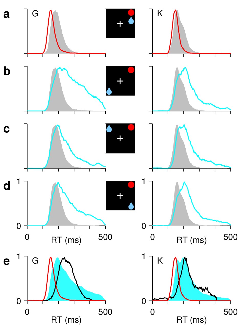
Asymmetric reward expectation leads to strong spatial bias.

(a–d) RT distributions for correct saccades, for monkeys G (left column) and K (right column). Insets indicate rewarded location (blue drop) and target (red circle). When the two are congruent ([a], red traces), RTs are shorter and less variable than when they are incongruent, that is, either opposite ([b], cyan) or adjacent ([c], [d], cyan). In unbiased trials (ADR task; gray), results are intermediate. (e) RT distributions in correct congruent (red, same data as in [a]), correct incongruent (cyan, data in [b-d] combined), and incorrect incongruent (black) trials. Histograms are normalized to a maximum of 1. The RTs during errors are neither the fastest nor the slowest.

https://doi.org/10.7554/eLife.33456.004

Figure 2—figure supplement 1

Download asset Open asset

Variations in spatial bias over time.

Analyses of the sequential responses made by the two animals confirmed that they were strongly aware of which location was the rewarded one. (a, b) Time course of bias adaptation after a change in rewarded location. Mean RT ( $\pm$ 1 SE) for saccades to a fixed location as a function of the number of trials before or after a change in reward status (i.e., block transition). Transitions from unrewarded to rewarded (a, red) are faster than from rewarded to unrewarded (b, cyan). Horizontal lines indicate asymptotic RT values. Black lines are exponential fits with time constants as indicated ( $τ$ ; units are trials). (c, d) Trial history effects. Mean RTs ( $\pm$ 1 SE) to rewarded ([c], red) and unrewarded ([d], cyan) targets are shown conditioned on various preceding sequences of rewarded (R) and unrewarded (U) trials. Note systematic changes in RT, which are somewhat idiosyncratic to each animal, as each condition is repeated. For calculating these trial-history effects, the first 15 trials after each block transition were excluded. All data are from correct responses.

https://doi.org/10.7554/eLife.33456.005

Figure 2—figure supplement 2

Download asset Open asset

Impact of reward-location bias on saccade metrics.

All plots compare measurements in congruent (red labels and markers) versus incongruent conditions (blue labels and markers). (a) Endpoints of saccades to a stimulus located at (10 $^{\circ}$ , 0 $^{\circ}$ ) collected during a single session from monkey G. The origin corresponds to the average saccade endpoint. For each data point, the displacement is the distance to the origin. Yellow circles indicate 1 and 2 SDs in displacement from the congruent data. (b) Mean normalized displacement in each experimental session ( $n = 135$ ). Displacement values for each session were z-scored, and then congruent and incongruent trials were averaged separately. Colors indicate monkeys (G, gray; K, white). The session shown in (a) is marked by the green cross. (c) Mean normalized displacement for each monkey, averaged across sessions. Error bars indicate $\pm$ 1 SE. (d) Average time course of eye velocity for saccades to stimuli at (8 $^{\circ}$ , 4 $^{\circ}$ ) collected during a single session from monkey K. Inset zooms in on the change in peak velocity of $\sim 40^{\circ}$ /s between congruent (red, $n = 104$ trials) and incongruent (blue, $n = 427$ trials) trials. Shades indicate $\pm$ 1 SE across trials. (e) Mean peak velocity in each experimental session. Colors indicate monkeys (G, gray; K, white). The session shown in (d) is marked by the green cross. (f) As in (e) but for saccade amplitude. (g) Average velocity (top) and amplitude (bottom) values averaged across sessions and monkeys. Error bars indicate $\pm$ 1 SE. All significance values are for differences in means across experimental conditions, from permutation tests for paired data. The results indicate that saccades to high-reward locations are spatially more precise (a–c) and have higher peak velocities (d, e, g) than those to low-reward locations, whereas saccade amplitude changes little in comparison (f, g). Results are consistent with earlier reports (Lauwereyns et al., 2002; Takikawa et al., 2002; Watanabe and Hikosaka, 2005).

https://doi.org/10.7554/eLife.33456.006

Figure 3 with 1 supplement

Download asset Open asset

Baseline activity predicts response gain, threshold, and outcome.

(a–c) Normalized firing rate as a function of time for a population of 62 neurons ( $V$ , $VM$ , and $M$ ) for which both correct and incorrect responses were collected. Icons indicate target (red circle), rewarded location (blue drop), and saccade (white cross) relative to the RF (gray area) in each case. Paired reddish and greenish traces correspond to activity with the target inside or outside the RF, respectively, in the same behavioral condition. For congruent trials (a) only correct responses are shown. For incongruent trials both correct (b) and incorrect (c) responses are shown. The reference line (dotted) is identical across panels. (d) (e) Mean peak activity (d) and mean baseline activity (e) for each target-reward-saccade (TRS) combination, from the same 62 neurons in (a–c). Error bars indicate $\pm 1$ SE across cells. (f) Baseline activity (z-scored) for incorrect (y axis) versus correct outcomes (x axis) under identical target and reward conditions. Each point is one neuron. Magenta dots indicate IOO versus IOI trials (target in/reward out); cyan dots indicate OII versus OIO trials (target out/reward in).

https://doi.org/10.7554/eLife.33456.007

Figure 3—figure supplement 1

Download asset Open asset

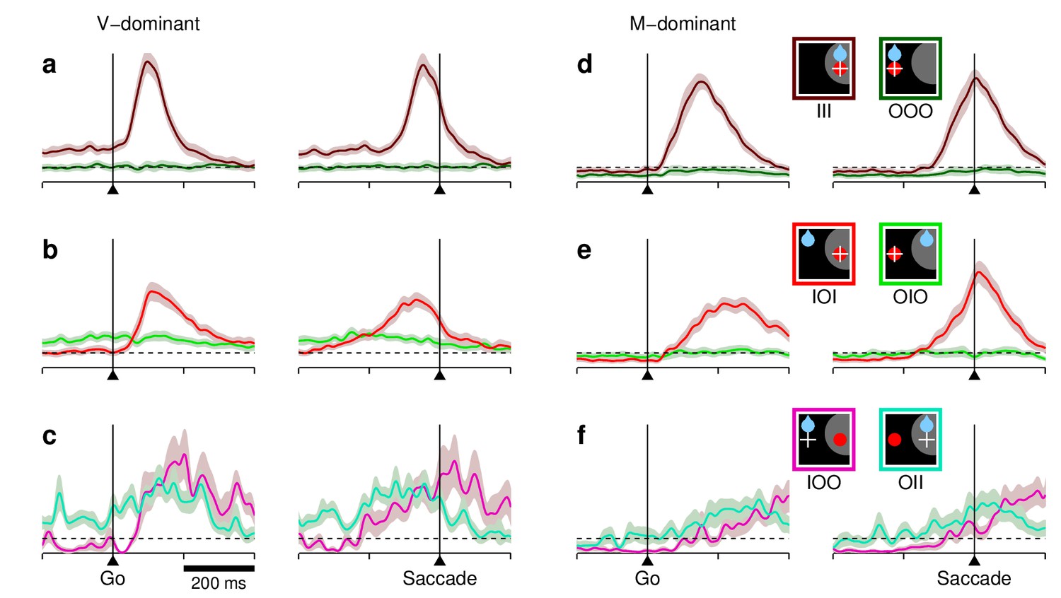
Responses of predominantly visual and predominantly movement-related neurons in FEF across conditions and outcomes.

Each panel shows normalized firing rate as a function of time for different combinations of target (red circle), reward (blue drop), and saccade (white cross) locations relative to the RF (gray area), as indicated by the icons on the right. The dotted reference line is the same for all panels. (a–c) Results are as in Figure 3a–c, except that they are based on the 33% of the cells ( $n = 21$ ) that were most visual, that is, had the lowest visuomotor index values. (d–f) As in panels (a–c) except that the results are based on the 33% of the cells ( $n = 21$ ) that were most motor, that is, had the highest visuomotor index values. Note differences in timing and in absolute baseline levels between visual and movement-related traces, but the similar relationships between motor plans into and away from the RF across conditions.

https://doi.org/10.7554/eLife.33456.008

Figure 4

Download asset Open asset

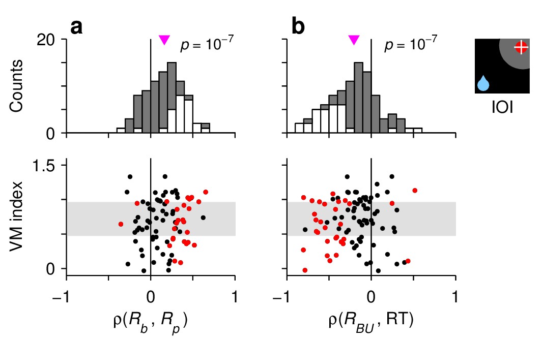
Characteristic manifestations of the rise-to-threshold process in single FEF neurons.

Each panel shows Spearman correlation coefficients calculated for 90 $V$ , $VM$ , and $M$ neurons. (a) Correlations between baseline activity and peak response. (b) Correlations between build up-rate and RTals. In each panel, the scatterplot (bottom) shows the same correlation coefficients as the histogram (top) but together with the visuomotor indices of the neurons. Gray shades in the scatterplots demarcate the borders defining the $V$ , $VM$ , and $M$ cell categories. White bars in histograms and red points in scatterplots indicate significant correlations ( $p < 0.05$ ). Pink triangles mark mean values, with significance from a signed-rank test indicated.

https://doi.org/10.7554/eLife.33456.009

Figure 5 with 1 supplement

Download asset Open asset

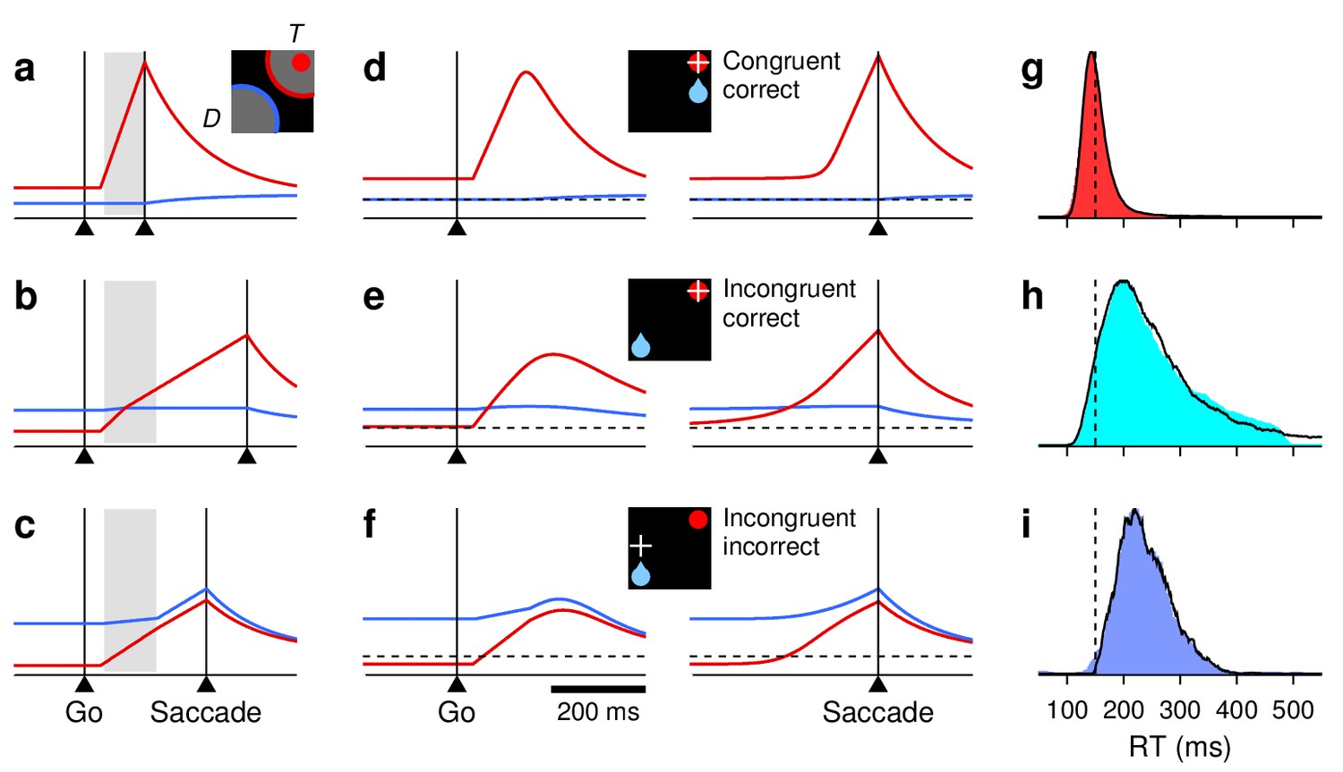
Simulation results from a saccadic competition model that bridges the neural and behavioral data.

(a–c) Simulated activity in three single trials. Traces show motor plans toward the target location ( $T$ , red) and the diametrically opposite location ( $D$ , blue). Gray shades mark the period during which the target stimulus suppresses the motor plan toward $D$ . When the target-driven activity, $R_{T}$ (red), reaches threshold first (a, b), the saccade is correct; when the bias-driven activity, $R_{D}$ (blue), reaches threshold first (c), the saccade is incorrect. The scale on the y axes is the same for all three plots. (d–f) Mean firing rate traces $R_{T}$ (red) and $R_{D}$ (blue) averaged across correct congruent (d), correct incongruent (e), and incorrect incongruent (f) simulated trials. Same format as in Figure 3a–c. (g–i) RT distributions from the same simulations as in panels (d–f), with trials sorted accordingly: for correct congruent (g), correct incongruent (h), and incorrect incongruent (i) trials. Colored shades are combined data from the two monkeys; black lines are model results. Dotted vertical lines at 150 ms are for reference.

https://doi.org/10.7554/eLife.33456.010

Figure 5—figure supplement 1

Download asset Open asset

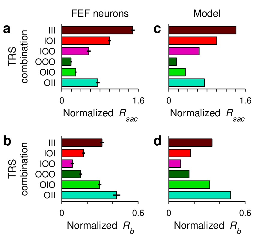
Variations in baseline and threshold levels in FEF and in the saccadic competition model.

(a) Mean normalized activity preceding saccade onset, $R_{s a c}$ , for each target-reward-saccade (TRS) combination. Data are from the same population and in the same format as those in Figure 3d, but here activity is based on the firing rate of each neuron computed in a fixed 50 ms window ending at saccade onset. Also, each unit’s responses were normalized before averaging across cells. Error bars indicate $\pm 1$ SE across cells. (b) Mean baseline activity (preceding the go signal), $R_{b}$ , for each experimental condition. Data are from the same population and in the same format as those in Figure 3e, but here each unit’s responses were normalized by the same factor as in (a) before averaging across cells. (c, d), As (a) and (b) but from model simulations; same runs as in Figure 5d–f. Presaccadic activity, $R_{s a c}$ , was equated to the response at threshold crossing. Baseline activity, $R_{b}$ , was equated to the response at the go signal. To compare the FEF and model responses in the same scale, both data sets were rescaled so that $R_{s a c}$ in the IOI condition was equal to 1.

https://doi.org/10.7554/eLife.33456.011

Figure 6 with 1 supplement

Download asset Open asset

Disentangling the coupling between baseline activity, build-up rate, and threshold.

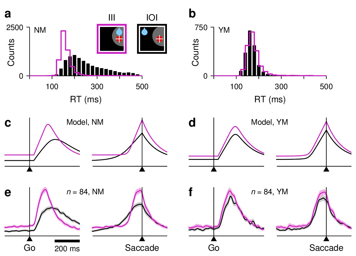
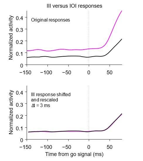
(a) Original RT distributions for III (magenta) and IOI (black) trials from all FEF recording sessions (non-matched condition, NM). (b) RT distributions after RT matching (yes-matched condition, YM). (c), Firing rate as a function of time for the target-driven activity, $R_{T}$ , in simulated III (magenta) and IOI (black) trials; same as red traces in Figure 5d,e. RTs are not matched. (d) As (c), but with matched RTs. (e) Normalized firing rate as a function of time for a population of 84 $V$ , $VM$ , and $M$ neurons. RTs are not matched. (f) As (e) but with matched RTs.

https://doi.org/10.7554/eLife.33456.012

Figure 6—figure supplement 1

Download asset Open asset

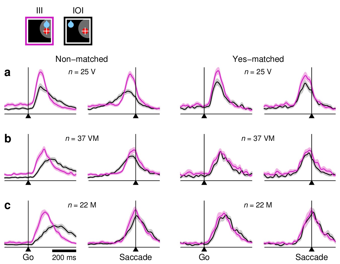
Comparisons between congruent and incongruent conditions, with and without RT equalization, for individual cell types.

Each panel shows normalized firing rate as a function of time in III (magenta) versus IOI (black) trials. Plots on the left include all recorded trials in each condition (non-matched), whereas plots on the right only include trials with matched RTs (yes-matched). The format is the same as in Figure 6e,f. (a) Responses of 25 $V$ neurons. (b) Responses of 37 $VM$ neurons. (c) Responses of 22 $M$ neurons. The effect of RT matching is qualitatively similar for the three cell types.

https://doi.org/10.7554/eLife.33456.013

Figure 7 with 3 supplements

Download asset Open asset

RT sensitivity of the average population activity.

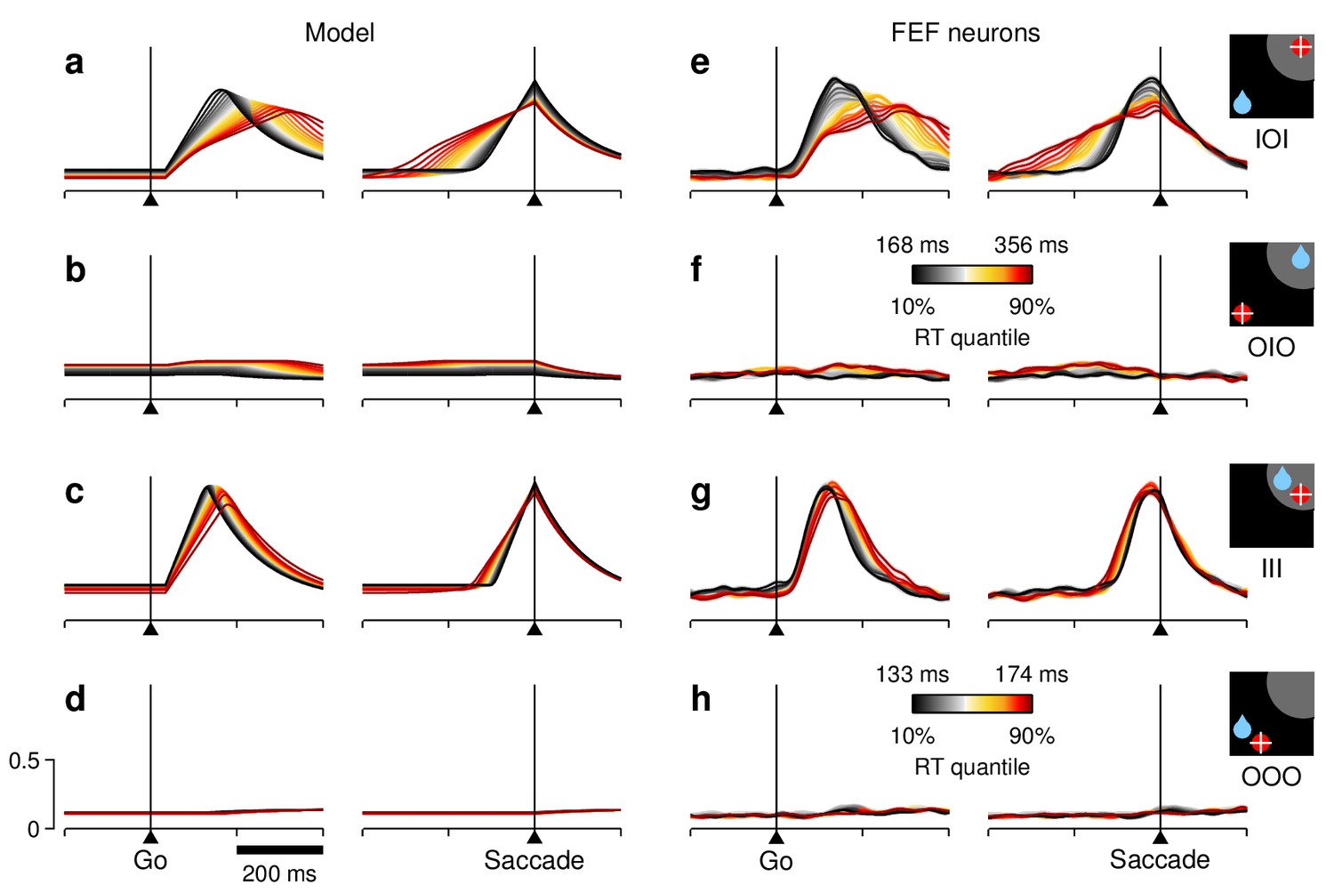
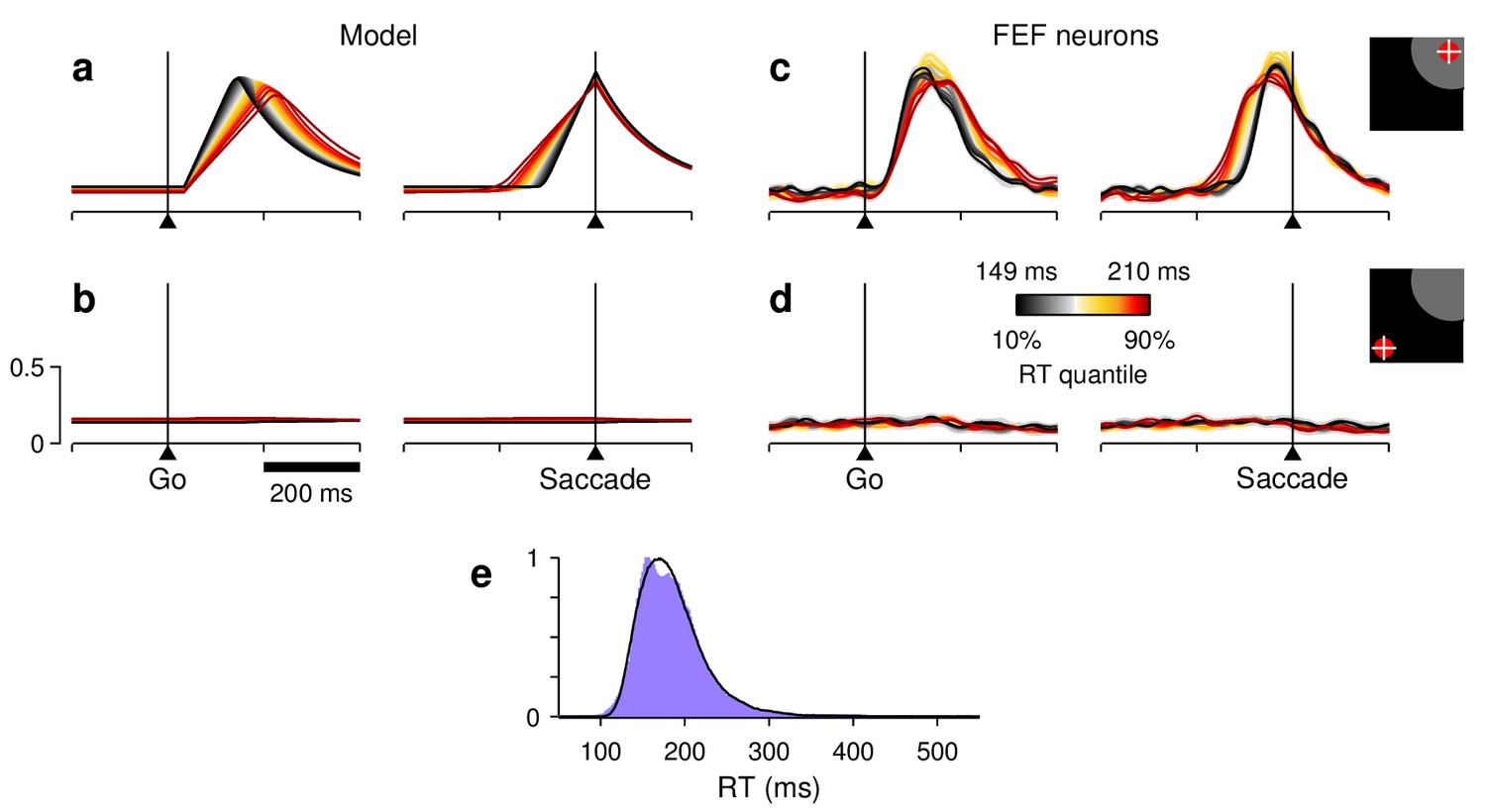
(a–d) Firing rate as a function of time for the simulated motor plans $R_{T}$ (a, c) and $R_{D}$ (b, d) during incongruent (a, b) and congruent (c, d) trials. The corresponding experimental conditions are indicated by the icons (far right). Curves are based on the same simulations as in Figure 5d–f. Each colored trace includes 20% of the simulated trials around a particular RT quantile. (e–h) Normalized firing rate as a function of time for a population of 84 FEF neurons ( $V$ , $VM$ , and $M$ ). Activity is for correct saccades in the four experimental conditions indicated. Each colored trace includes 20% of the trials recorded from each participating cell around a particular RT quantile. Lighter shades behind lines indicate $\pm$ 1 SE across cells. Color bars apply to both simulated and recorded data in incongruent (color bar in [f]) or congruent conditions (color bar in [h]). The scale bars in (d) apply to all panels.

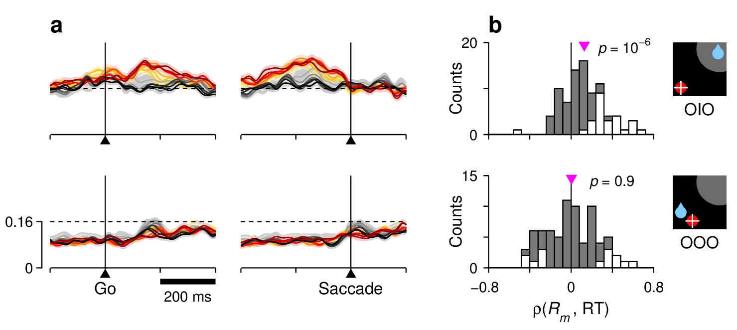
https://doi.org/10.7554/eLife.33456.014

Figure 7—figure supplement 1

Download asset Open asset

Correlation between RT and activity during correct saccades away from the RF.

For each row, the corresponding target-reward-saccade configuration is depicted by the icon on the far right. (a) Normalized neural responses. Each colored trace corresponds to population firing rate as a function of time for a subset of trials around a particular RT quantile. Traces are the same as in Figure 7f,h, but with a shorter scale on the y axes, as marked on the bottom panel. The dashed reference line is identical across panels. (b) Distributions of Spearman correlation coefficients between RT and mean activity, $ρ (R_{m}, RT)$ , where $R_{m}$ is the mean response between the go signal and saccade onset. The data in each histogram are from the same 84 cells used in Figure 7. White bars correspond to significant correlations ( $p < 0.05$ ). Pink triangles mark mean values, with significance from signed-rank tests shown next to them.

https://doi.org/10.7554/eLife.33456.015

Figure 7—figure supplement 2

Download asset Open asset

RT sensitivity of the $VM$ / $M$ population activity.

The format is exactly the same as in Figure 7, except that the results are based only on the activity of the cells classified as $VM$ and $M$ ; that is, all of the $V$ neurons ( $n = 26$ , visuomotor index $<$ 0.46) were excluded. The resulting population averages (e–h) showed only slight differences with respect to the averages obtained with the larger neuronal sample. For the simulations shown (a–d), the model parameters were adjusted so that the model matched those slight differences in activity, while still replicating the corresponding RT distributions.

https://doi.org/10.7554/eLife.33456.016

Figure 7—figure supplement 3

Download asset Open asset

Responses in the ADR task, in which all correct trials were equally rewarded.

(a,b) Firing rate as a function of time for the motor plans $R_{T}$ (a) and $R_{D}$ (b) during simulated ADR trials. Colors correspond to RT quantiles, as in previous figures. (c, d) Normalized firing rate as a function of time for a population of 38 FEF neurons ( $V$ , $VM$ , and $M$ ) recorded in the ADR task. Activity is for correct saccades into (c) or away from (d) the cells’ RFs, as indicated. (e) RT distributions obtained from the ADR recording sessions (purple shade) and from the simulations (black trace). Model results were generated with the same parameters used to simulate the IOI and III trials in the 1DR task, with three exceptions: the two mean baseline values were equal and less variable ( $B_{T} = B_{D} = 0.2$ and $σ = 0.14$ in Equation 5), and the build-up rate of the stimulus-driven response was slightly lowered (by setting the first term in Equation 5 equal to 5.95 instead of 6.16). Otherwise, the model simulations proceeded exactly as described for the 1DR task.

https://doi.org/10.7554/eLife.33456.017

Figure 8

Download asset Open asset

Correlation between RT and baseline activity in FEF.

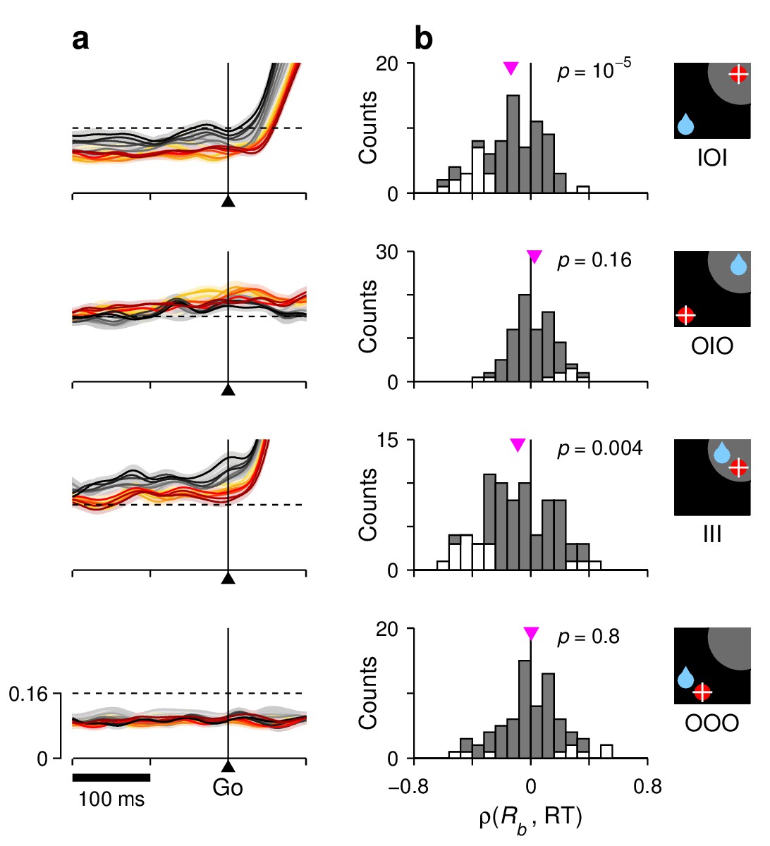
For each row, the corresponding target-reward-saccade configuration is depicted by the icon on the far right. (a) Normalized neural responses around the go signal. Each colored trace corresponds to population firing rate as a function of time for a subset of trials around a particular RT quantile. Traces are exactly as in Figure 7e–h (left panels), except at shorter x and y scales, as marked on the bottom panel. The dashed reference line is identical across panels. (b) Distributions of Spearman correlation coefficients between RT and baseline activity, $ρ (R_{b}, RT)$ . The data in each histogram are from the same cells used in Figure 7. White bars correspond to significant correlations ( $p < 0.05$ ). Pink triangles mark mean values, with significance from signed-rank tests indicated.

https://doi.org/10.7554/eLife.33456.018

Figure 9

Download asset Open asset

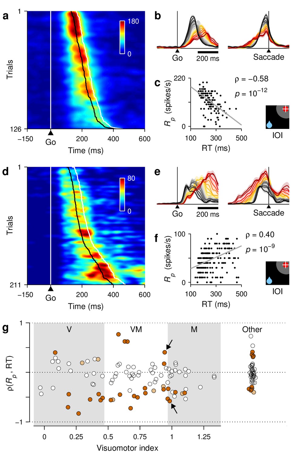
RT sensitivity of individual FEF neurons.

(a–c) Responses of a single FEF cell that fired preferentially during short RTs. All data are from IOI trials (icon). (a) Activity map. Each row corresponds to one trial, and shows the cell's firing rate (represented by color) as a function of time (x axis) with spikes aligned to the go signal (vertical white line). Trials are ordered by RT from fastest (top) to slowest (bottom). For this cell, the time of peak activity (black marks) closely tracks saccade onset (white marks). (b) Firing rate as a function of time, with trials sorted and color-coded by RT, as in Figure 7. (c) Peak response as a function of RT. Each dot corresponds to one trial. The gray line shows linear fit. Numbers indicate Spearman correlation $ρ (R_{p}, RT)$ and significance. (d–f) As (a–c) but for a single cell that fired preferentially during long RTs. (g) Spearman correlation between peak response and RT for all classified cells ( $n = 132$ ). For standard cell types ( $V$ , $VM$ , $M$ ), values on the abscissa correspond to visuomotor index; for other cells, they are arbitrary. Shades demarcate ranges approximately corresponding to standard $V$ , $VM$ , and $M$ categories. All correlation values are from IOI trials. Brown points indicate significant neurons (light, $p <$ 0.05; dark $p < 0.01$ ). Arrows identify example cells in panels above.

https://doi.org/10.7554/eLife.33456.019

Figure 10

Download asset Open asset

RT sensitivity in subpopulations of FEF neurons.

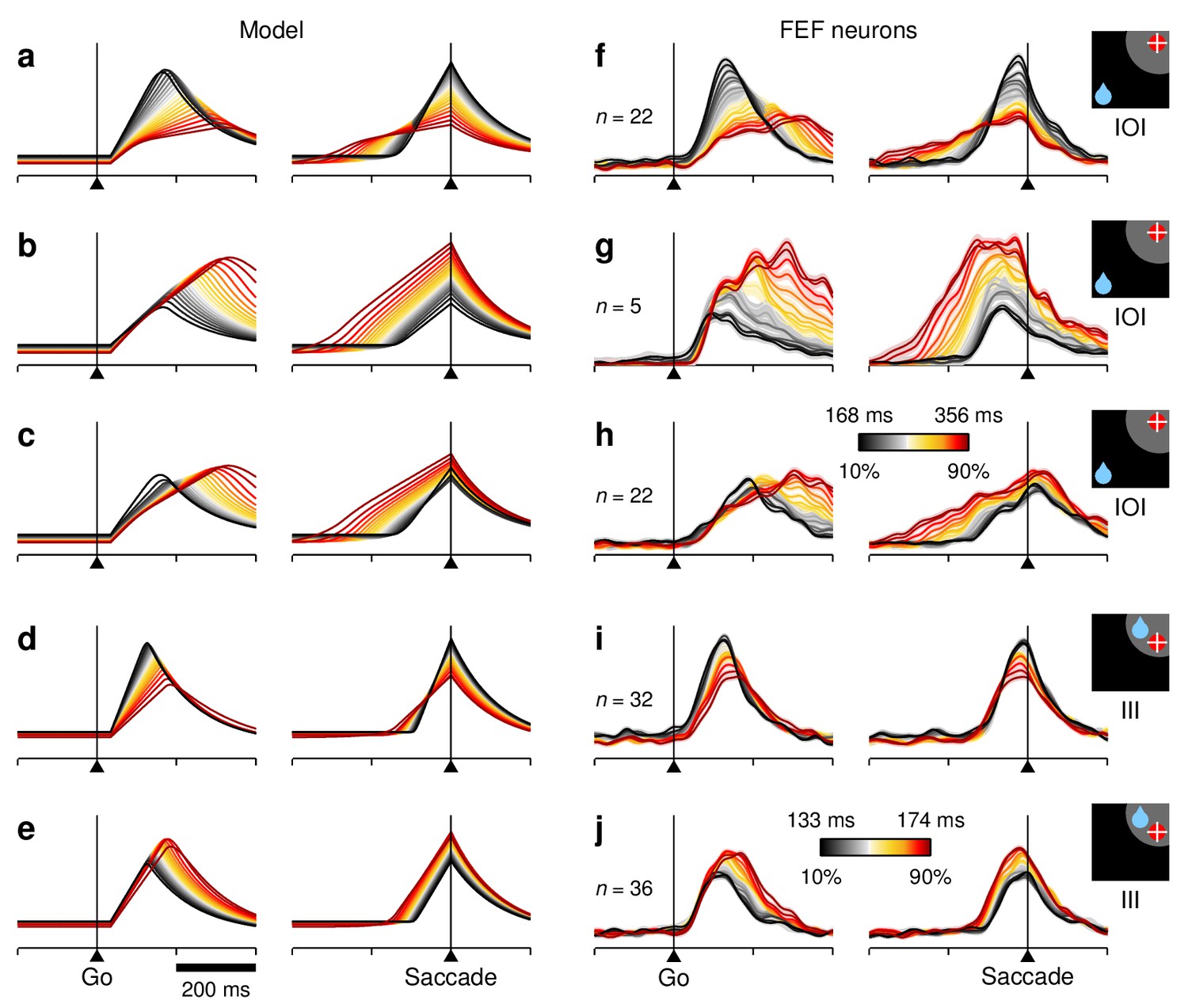
All panels show firing rate as a function of time, with each colored curve based on a different subset of trials selected according to RT, as in Figure 7. Only activity associated with correct saccades into the RF is displayed. (a–e) Simulated activity demonstrating a clear preference for either short (a, d) or long RTs (b, c, e). The model generated fast- and slow-preferring responses in both IOI (a–c) and III trials (d, e) with varying modulation strengths. (f–j) As in (a–e) but based on the responses of various subsets of FEF neurons with similar RT preferences, as quantified based on $ρ (R_{p}, RT)$ . Each subset is a selection from the same pool of 84 recorded neurons used in Figure 7 (in [f] $ρ < 0$ and $p < 0.05$ ; in [g] $ρ > 0$ and $p < 0.05$ ; in [h] $ρ > 0$ ; in (i) $ρ < 0$ ; in [j] $ρ > 0$ ; visuomotor index $> 0.4$ in all cases). Numbers of participating cells are indicated in each panel. Lighter shades behind lines indicate $\pm$ 1 SE across cells. Color bars apply to both simulated and recorded data, either in IOI (color bar in h) or III trials (colorbar in j).

https://doi.org/10.7554/eLife.33456.020

Author response image 1

Download asset Open asset

https://doi.org/10.7554/eLife.33456.026

Additional files

Source code 1 Matlab script for simulating the simplest version of the saccadic competition model. This script generates RT distributions and average $R_{T}$ and $R_{D}$ traces as functions of time (as in Figure 5).: https://doi.org/10.7554/eLife.33456.021
Download elife-33456-code1-v2.m
Source code 2 Matlab script for simulating the saccadic competition model with two types of target-driven response. This script works in the same way as Source code 1, except that $R_{T}$ is split into separate $R_{T}^{C}$ and $R_{T}^{U}$ components (as defined in Equation 1).: https://doi.org/10.7554/eLife.33456.022
Download elife-33456-code2-v2.m
Source code 3 Matlab script for sorting the response traces produced by Source code 1 and 2 into RT quantiles (as in Figures 7 and 10).: https://doi.org/10.7554/eLife.33456.023
Download elife-33456-code3-v2.m
Transparent reporting form: https://doi.org/10.7554/eLife.33456.024
Download elife-33456-transrepform-v2.docx

Download links

A two-part list of links to download the article, or parts of the article, in various formats.

Downloads (link to download the article as PDF)

Open citations (links to open the citations from this article in various online reference manager services)

Mendeley

Cite this article (links to download the citations from this article in formats compatible with various reference manager tools)

Christopher K Hauser
Dantong Zhu
Terrence R Stanford
Emilio Salinas

(2018)

Motor selection dynamics in FEF explain the reaction time variance of saccades to single targets

eLife 7:e33456.

https://doi.org/10.7554/eLife.33456

Sign up for email alerts

Privacy notice