Structure-based membrane dome mechanism for Piezo mechanosensitivity
- Howard Hughes Medical Institute, The Rockefeller University, United States
Figures
Figure 1
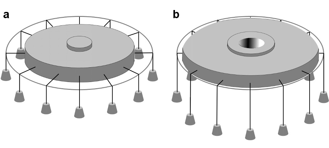
In-plane area expansion lowers the free energy of a channel-membrane system under tension.
Analog of a membrane under tension showing tethered weights in a gravitational field pulling the membrane taut, adapted from Ursell et al. (2008). (a) When the channel is closed, potential energy from the weights is high. (b) When the channel opens and in-plane area expands, the weights are lowered, and the potential energy of the system is decreased.
Figure 2 with 3 supplements
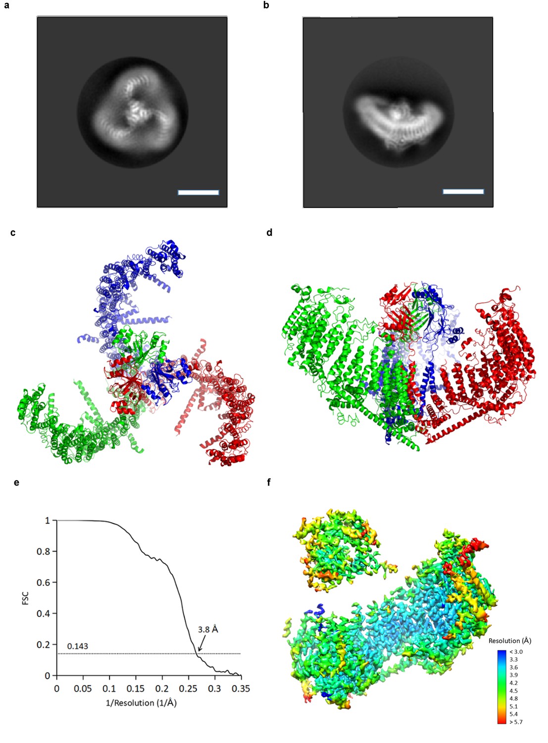
CryoEM reconstruction of mPiezo1.
(a and b) Representative 2D averaged classes, viewed from the top (a), and the side (b), scale bar 10 nm. (c and d) Atomic model of the trimeric channel shown as ribbon diagram, viewed from the top (c), and the side (d). The three subunits are colored in red, green and blue, respectively. (e) Fourier shell correlation (FSC) curves calculated between two half maps after C1 masked refinement and post-processing in RELION. (f) Local resolution of density map from C1 masked refinement, estimated by Blocres. The map shown is low-pass filtered to 3.8 Å and sharpened with a b-factor of −200 Å2.
Figure 2—figure supplement 1
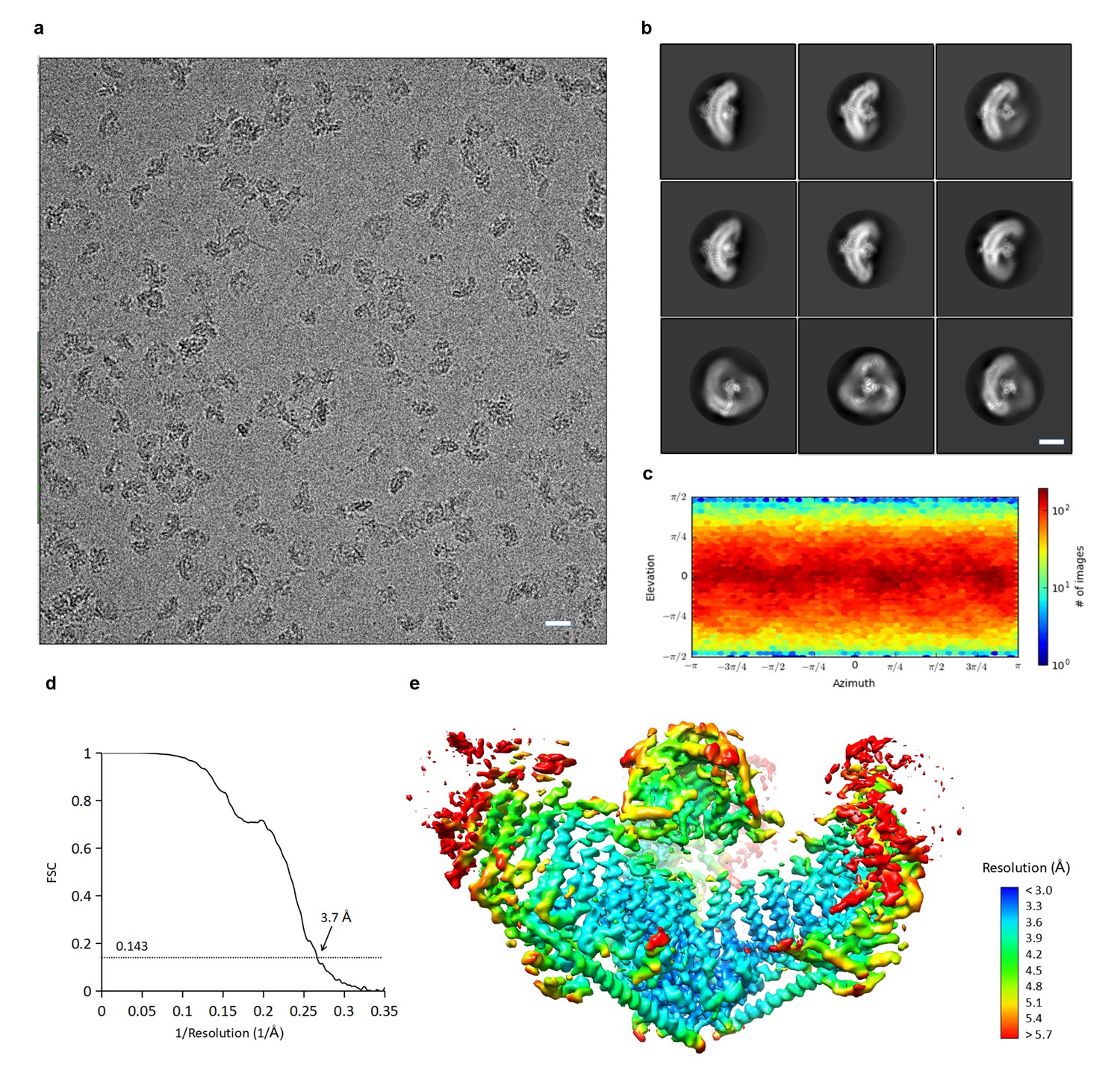
CryoEM structure determination of mPiezo1.
(a) Representative raw micrograph of mPiezo1. Scale bar 200 Å. (b) Selected 2D class averages representing different orientations of particles. Scale bar 10 nm. (c) Direction distribution over azimuth and elevation angles of particles used in CryoSPARC refinement. (d) Fourier shell correlation (FSC) curves between two half maps of CryoSPARC refinement with C3 symmetry imposed. (e) Local resolution of density map from C3 symmetry CryoSPARC refinement, estimated by Blocres. The map shown is sharpened with a b-factor of −122 Å2.
Figure 2—figure supplement 2
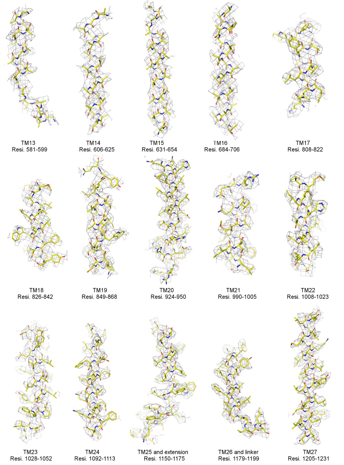
Local EM densities of mPiezo1 (Residues 581–1231).
Density map from RELION masked refinement in C1 symmetry was low-pass filtered to 3.8 Å, sharpened with a b-factor of −200 Å2, and contoured at 6σ. The atomic model is shown as sticks, colored according to atom type: yellow, carbon; red, oxygen; blue, nitrogen; and orange, sulfur.
Figure 2—figure supplement 3
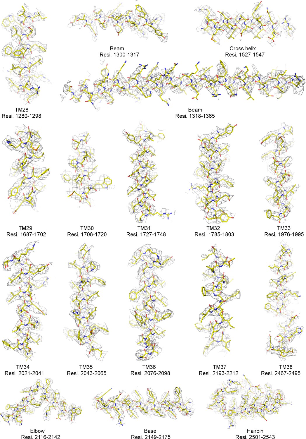
Local EM densities of mPiezo1 (Residues 1280–2543).
Density map from RELION masked refinement in C1 symmetry was low-pass filtered to 3.8 Å, sharpened with a b-factor of −200 Å2, and contoured at 6σ. The atomic model is shown as sticks, colored according to atom type: yellow, carbon; red, oxygen; blue, nitrogen; and orange, sulfur.
Figure 3 with 3 supplements
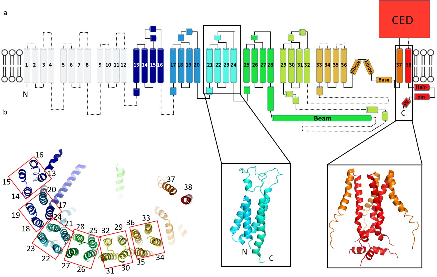
Topology of mPiezo1.
(a) Cartoon representation of a monomer, rainbow-colored with C-terminus in red and N-terminus in blue, except for the first 12 TMs that are not visible in our structure. Helices within a single 4-TM unit are colored uniquely. Helices are shown as cylinders, loops as solid lines, and unresolved regions as dotted lines. C-terminal extracellular domain (CED) is simplified as a box. A ribbon diagram of 4-TM unit 6, consisting of TM 21 to 24, is shown in the left inset panel with N- and C- termini labeled. The right inset panel shows a ribbon diagram of the pore region, formed by TM37, TM38 and the PE helix from all three subunits. (b) A ribbon diagram of a monomer rainbow-colored as in A, viewed from top. Each 4-TM unit is highlighted in a red box with TM number labeled.
Figure 3—figure supplement 1
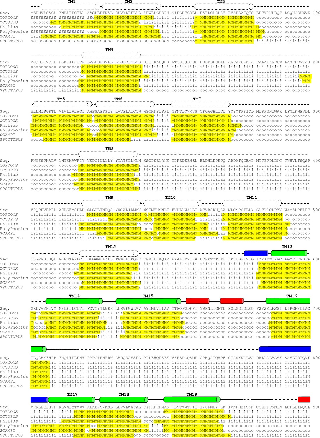
Hydrophathy analysis of mPiezo1 (Residues 1–900).
Transmembrane topology prediction was performed using TOPCONS (Tsirigos et al., 2015), OCTOPUS (Viklund and Elofsson, 2008), Philius (Reynolds et al., 2008), PolyPhobius (Käll et al., 2004), SCAMPI (Bernsel et al., 2008), SPOCTOPUS (Viklund et al., 2008). Predicted intracellular sequence is indicated by ‘i’, extracellular sequence by ‘o’, membrane region by ‘M’, and signal peptide by ‘S’. Predicted transmembrane sequence is highlighted in yellow. Secondary structures based on our structure are represented above the sequence as tubes (α-helices), arrows (β-sheets), or solid lines (loops). Regions not modeled in our structure are shown as dotted lines. The helices and sheets are colored in red (extracellular), blue (intracellular) or green (transmembrane).
Figure 3—figure supplement 2
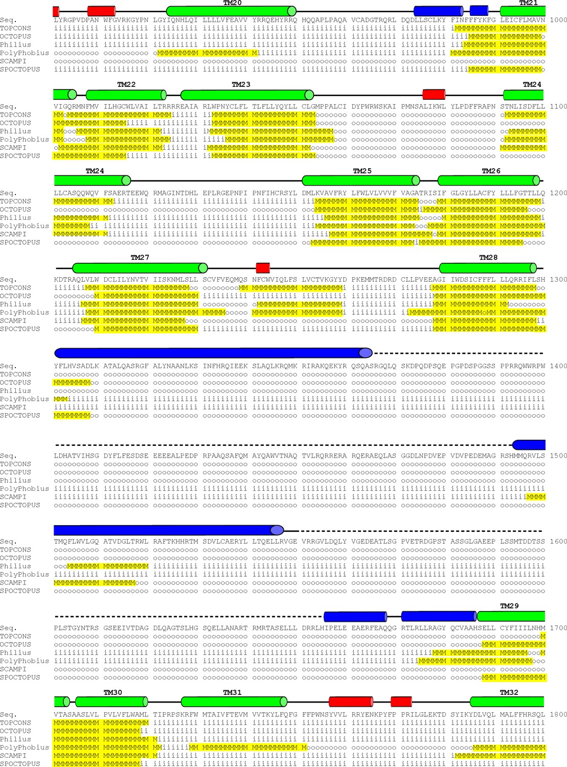
Hydrophathy analysis of mPiezo1 (Residues 901–1800).
Transmembrane topology prediction was performed using TOPCONS (Tsirigos et al., 2015), OCTOPUS (Viklund and Elofsson, 2008), Philius (Reynolds et al., 2008), PolyPhobius (Käll et al., 2004), SCAMPI (Bernsel et al., 2008), SPOCTOPUS (Viklund et al., 2008). Predicted intracellular sequence is indicated by ‘i’, extracellular sequence by ‘o’, membrane region by ‘M’, and signal peptide by ‘S’. Predicted transmembrane sequence is highlighted in yellow. Secondary structures based on our structure are represented above the sequence as tubes (α-helices), arrows (β-sheets), or solid lines (loops). Regions not modeled in our structure are shown as dotted lines. The helices and sheets are colored in red (extracellular), blue (intracellular) or green (transmembrane).
Figure 3—figure supplement 3

Hydrophathy analysis of mPiezo1 (Residues 1801–2547).
Transmembrane topology prediction was performed using TOPCONS (Tsirigos et al., 2015), OCTOPUS (Viklund and Elofsson, 2008), Philius (Reynolds et al., 2008), PolyPhobius (Käll et al., 2004), SCAMPI (Bernsel et al., 2008), SPOCTOPUS (Viklund et al., 2008). Predicted intracellular sequence is indicated by ‘i’, extracellular sequence by ‘o’, membrane region by ‘M’, and signal peptide by ‘S’. Predicted transmembrane sequence is highlighted in yellow. Secondary structures based on our structure are represented above the sequence as tubes (α-helices), arrows (β-sheets), or solid lines (loops). Regions not modeled in our structure are shown as dotted lines. The helices and sheets are colored in red (extracellular), blue (intracellular) or green (transmembrane).
Figure 4 with 1 supplement

mPiezo1 trimer in curved micelle.
(a) The same ribbon diagram of a monomer taken from the trimer, as in 3B, viewed from the side, with N- and C- termini labeled. Approximate locations of planar membrane interfaces are shown as grey lines. (b) Ribbon diagrams of a trimer in an unsharpened map, contoured at 6σ, showing micelle density. Top, side and bottom views are shown. (c) Surface representation of a trimer, colored based on electrostatic potentials in aqueous solution containing 150 mM NaCl, calculated using APBS, with positive shown blue, neutral white, and negative red. Top, side and bottom views are shown.
Figure 4—figure supplement 1
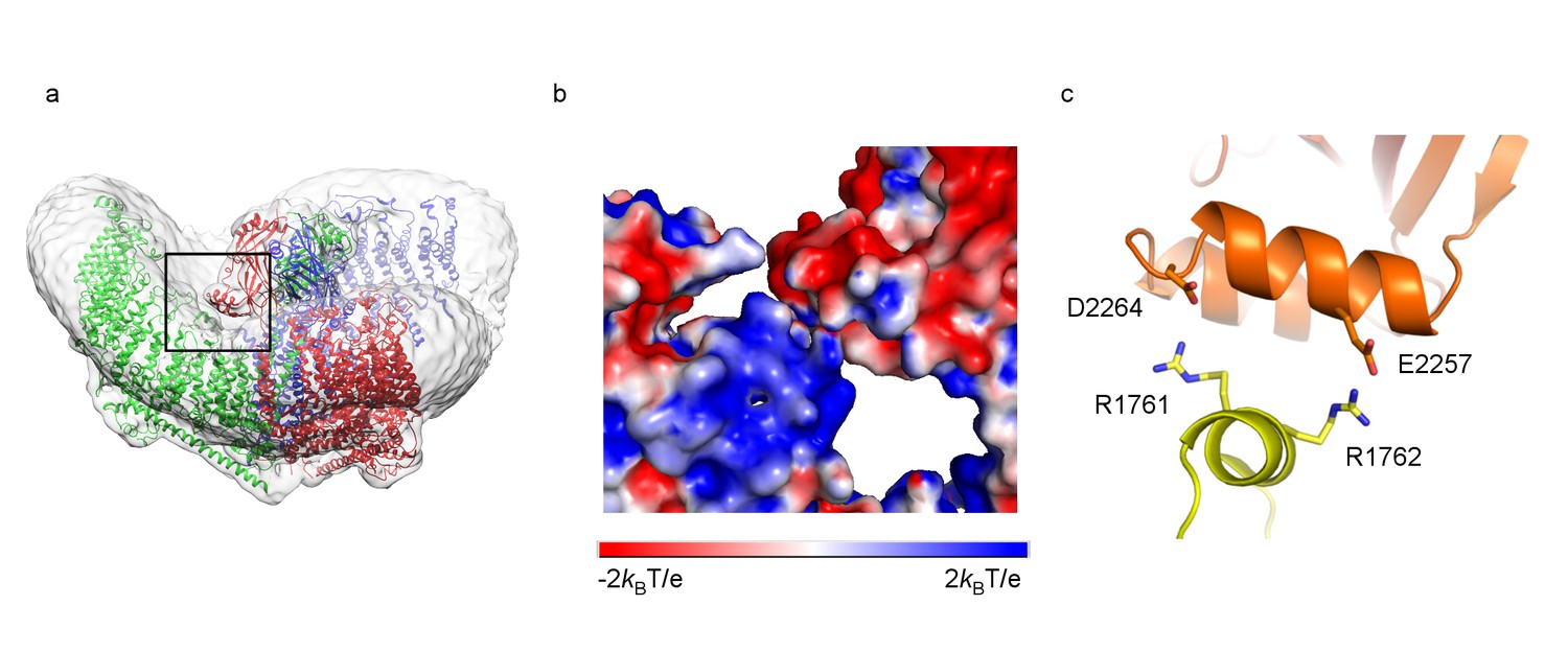
Interface between CED and TM loops.
(a) Ribbon diagram of a trimer in an unsharpened map. One of the three contact regions between CED and TM loops is highlighted in a black box. (b) Zoomed-in view of the region in black box in (a) as surface representation, colored based on electrostatic potentials in aqueous solution containing 150 mM NaCl, calculated using APBS, with positive in blue, neutral in white, and negative in red. (c) Ribbon diagram of the helices in contact, colored as in Figure 3. Interacting residues are shown as sticks.
Figure 5 with 1 supplement
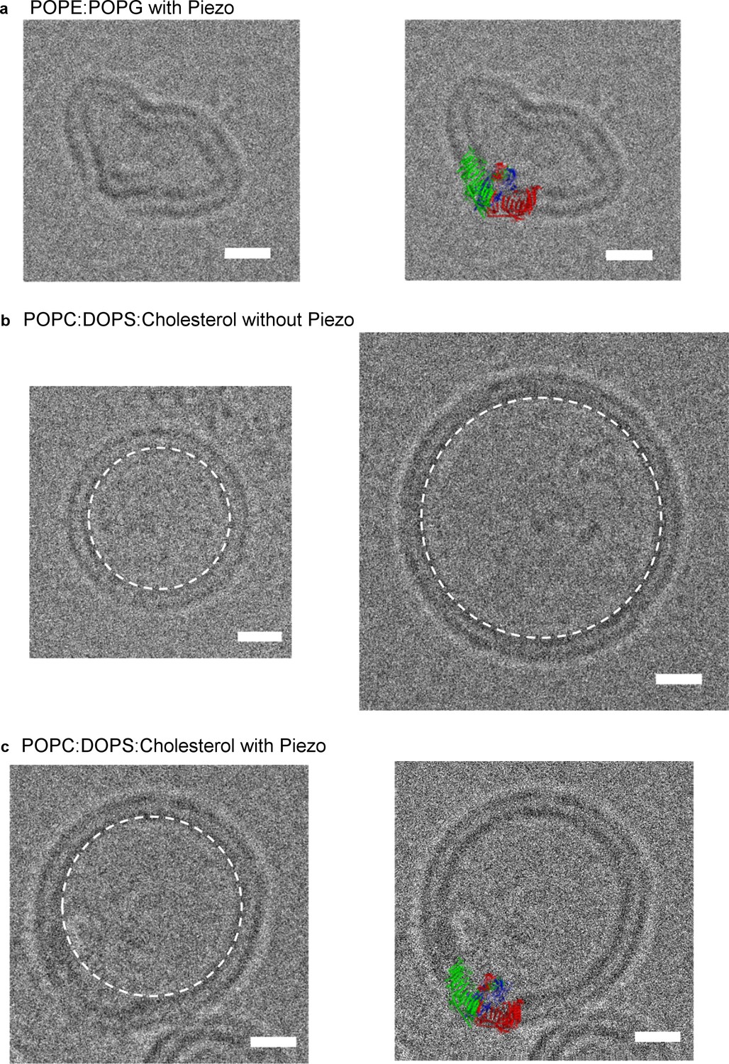
mPiezo1 trimer locally curves membrane.
(a) Small unilamellar vesicle containing Piezo without (left) and with (right) molecular model scaled to size and inserted into image. The lipid composition is POPE:POPG = 3:1 wt ratio. Scale bar 10 nm. (b) Small unilamellar vesicles containing no protein. The lipid composition is POPC:DOPS:cholesterol = 8:1:1 wt ratio. The spherical vesicle projection is highlighted by a white dashed circle. Scale bar 10 nm. (c) Small unilamellar vesicle containing Piezo without (left) and with (right) molecular model scaled to size and inserted into image. The lipid composition is POPC:DOPS:cholesterol = 8:1:1 wt ratio. The spherical vesicle projection is highlighted by a white dashed circle. Scale bar 10 nm.
Figure 5—figure supplement 1
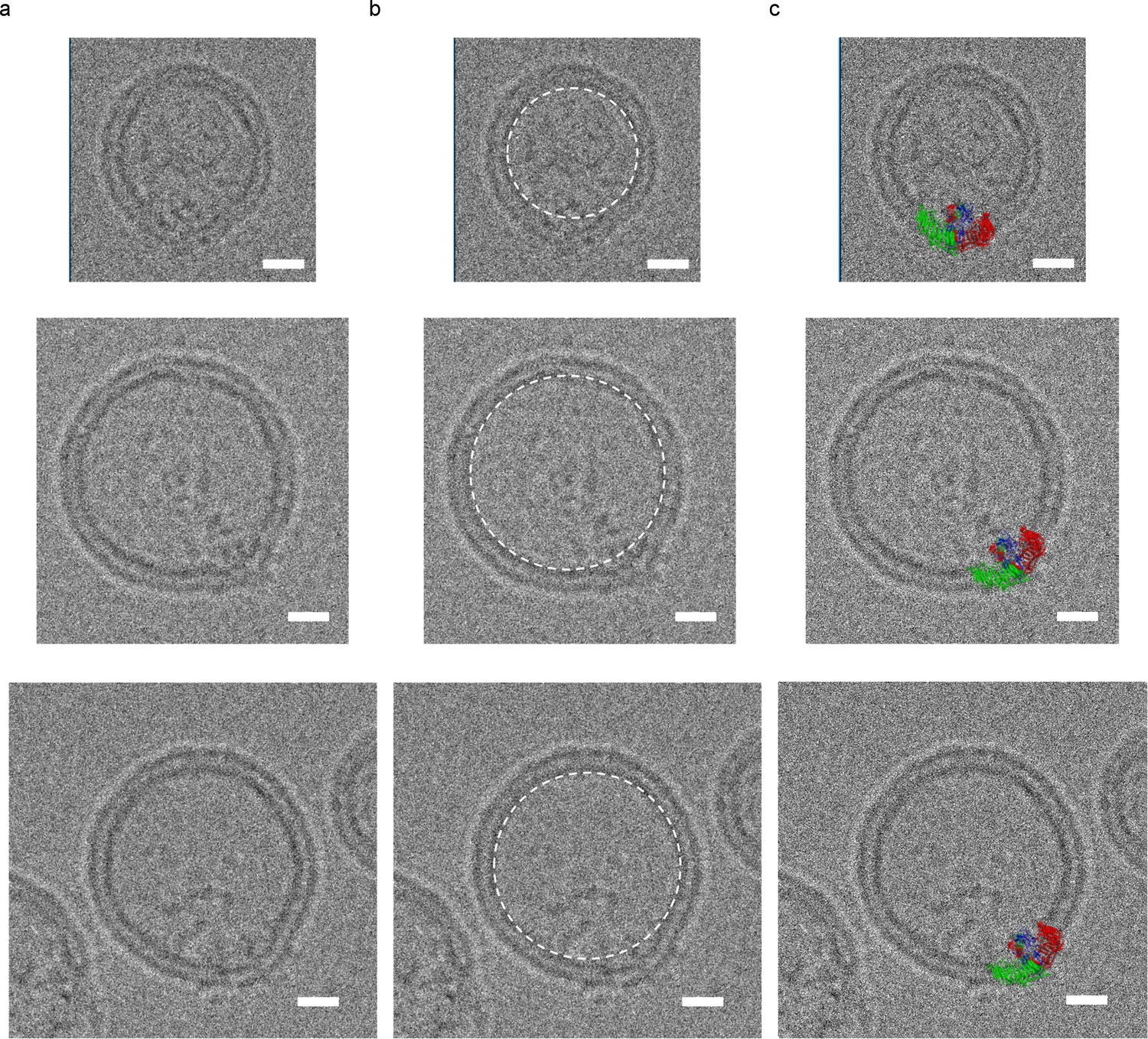
mPiezo1 trimer in liposomes of various sizes.
Small unilamellar vesicles containing Piezo. The lipid composition is POPC:DOPS:cholesterol = 8:1:1 wt ratio. Scale bar 10 nm. (a) The raw images. (b) Images with a white dashed circle highlighting the spherical vesicle projection. (c) Images with molecular model scaled to size and inserted into image.
Figure 6 with 1 supplement
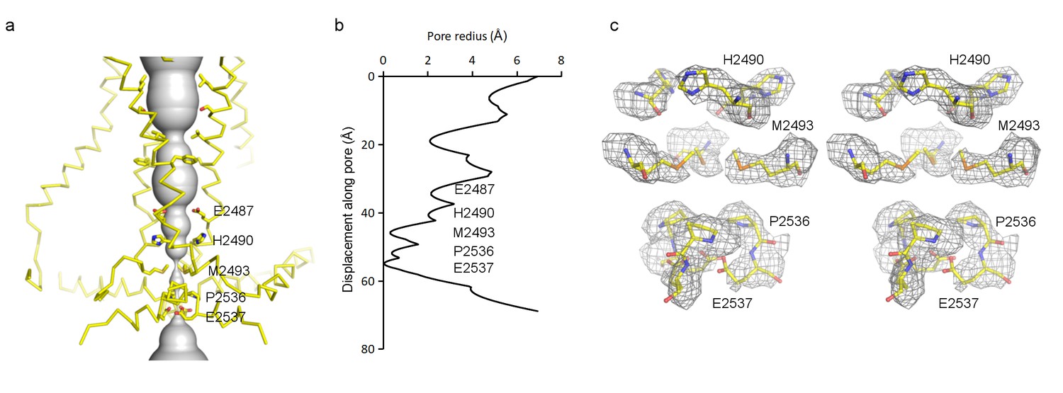
Pore of the mPiezo1 channel.
(a) Ion-conduction path viewed from the side. The distance from the pore axis to the protein surface is shown as grey sphere. Cα trace of the pore (TM37, TM38, hairpin and PE helices) is shown in yellow. Residues facing the pore are shown as sticks. Constricting residues are labeled. (b) Radius of the pore. The van der Waals radius is plotted against the distance from the top along the pore axis. Constricting residues are labeled as in A. (c) Stereo view of the side-chain density around constricting residues. The map is contoured at 6σ and sharpened with a b-factor of −200 Å2. The atomic model is shown as sticks, colored according to atom type: yellow, carbon; red, oxygen; blue, nitrogen; and orange, sulfur.
Figure 6—figure supplement 1
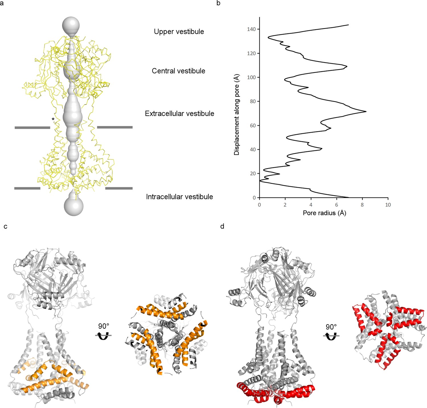
Pore region of the mPiezo1 channel.
(a) Potential ion-conduction path including the CED viewed from the side. The distance from the pore axis to the protein surface is shown as grey sphere. Cα trace of the pore region (residues 2116 to 2546) is shown in yellow. Estimated membrane interfaces on the basis of protein surface features are shown as grey lines. Four vestibules are labeled as in P2X and ASIC channels. Position of one of the fenestrations is indicated with an asterisk. (b) Radius of the potential ion-conduction pathway including the CED. The van der Waals radius is plotted against the distance from the bottom along the pore axis. (c) Ribbon diagram of the pore region in grey, with the elbow and triangular base helices highlighted in yellow. Both side view and bottom view are shown. (d) Ribbon diagram of the pore region in grey, with the hairpin and PE helices highlighted in red. Both side view and bottom view are shown.
Figure 7 with 1 supplement
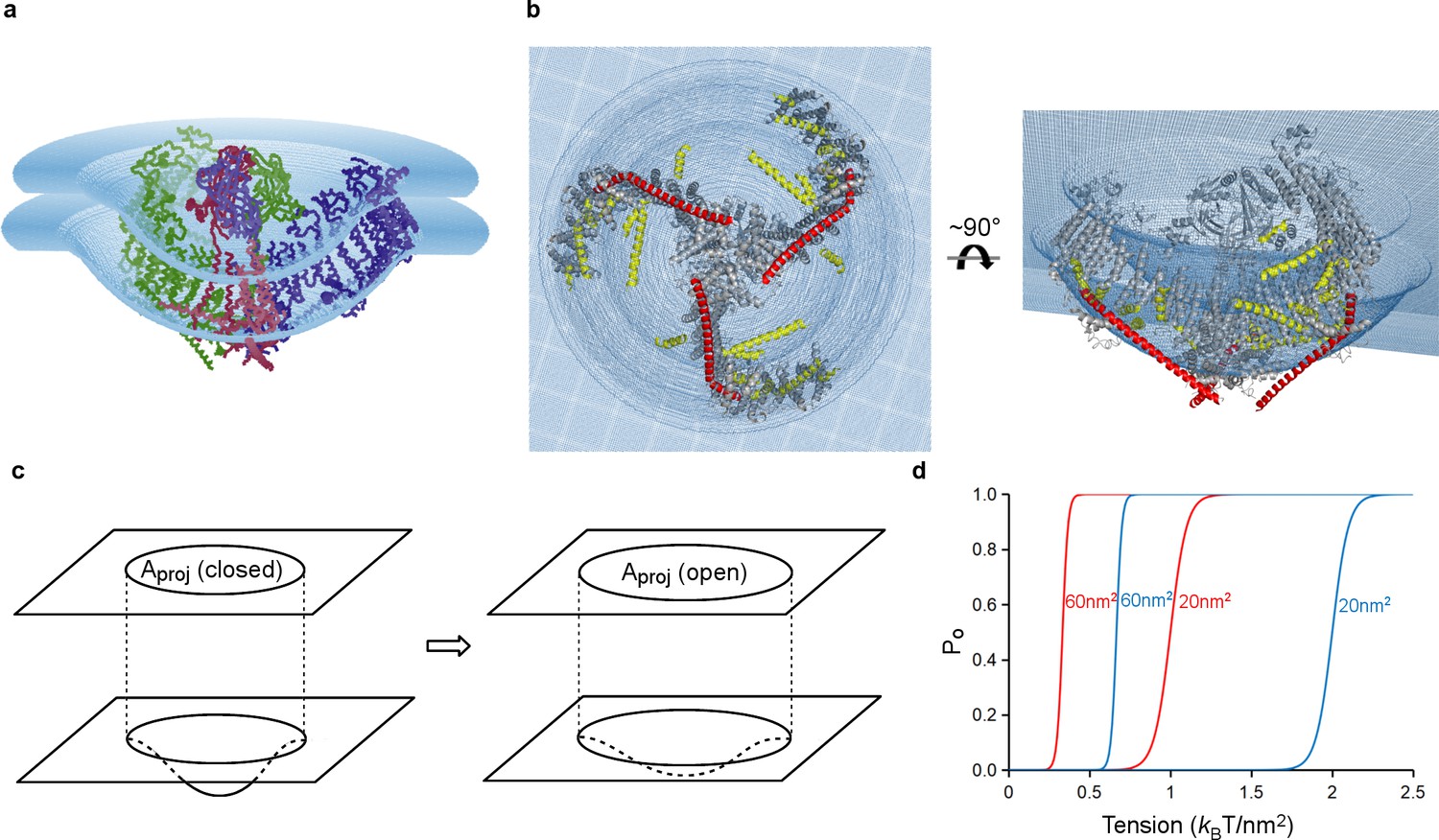
Model of tension-gating in mPiezo1.
(a) Cα trace representation of a trimer placed in a semi-sphere-shaped membrane 3.6 nm thick, idealized from the curved micelle density. The mid-plane semi-sphere has radius of 10.2 nm and is centered 4.0 nm above the projection plane. The three subunits are shown in red, green and blue, respectively. (b) Ribbon diagram of a trimer in the idealized membrane. The ‘beam’ formed by residues 1300–1365 is highlighted in red, the cross-helices are highlighted in yellow, while the remaining protein is colored in grey. (c) Illustration of projection area (circle in top plane) changing as the surface curvature of the channel and local membrane (bottom plane) changes. (d) Theoretical activation curves corresponding (ΔGprot + ΔGbend)=20 kBT (red) or 40 kBT (blue) and ΔAproj = 20 nm2 or 60 nm2. The curves are generated through Po = (1 + Exp[(ΔGprot + ΔGbend) - γΔAproj])−1.
Figure 7—figure supplement 1
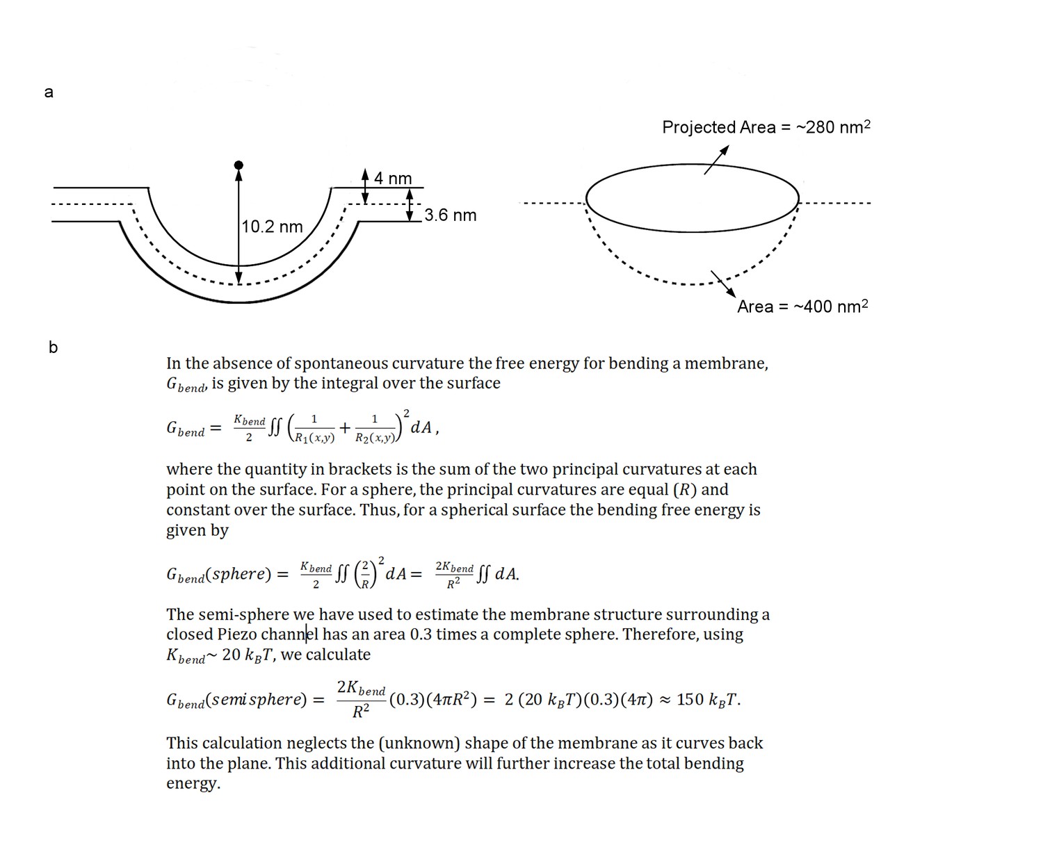
References for area and energy calculations.
(a) Schematic showing the semi-sphere-shaped membrane 3.6 nm thick, idealized from the curved micelle density. The mid-plane semi-sphere has radius of 10.2 nm and center 4.0 nm above the projection plane. Projected area and total mid-plane surface area are shown in the right panel. (b) Equations used for calculating the membrane bending energy (Rawicz et al., 2000; Helfrich, 1973; Deserno, 2007; Phillips, 2017).
Tables
Table 1
Cryo-EM data collection, refinement and validation statistics.
https://doi.org/10.7554/eLife.33660.007| mouse Piezo1 (EMDB-7042) (PDB 6B3R) | |
|---|---|
| Data collection and processing | |
| Magnification | 22,500 |
| Voltage (kV) | 300 |
| Electron exposure (e–/Å2) | 47 |
| Defocus range (μm) | 1.0–2.4 |
| Pixel size (Å) | 1.3 |
| Symmetry imposed | C1 |
| Initial particle images (no.) | 1 |
| Final particle images (no.) | 50 |
| Map resolution (Å) FSC threshold | 3.8 0.143 |
| Map resolution range (Å) | 3.2–10.7 |
| Refinement | |
| Initial model used (PDB code) | 4RAX |
| Map sharpening B factor (Å2) | −200 |
| Model composition Non-hydrogen atoms Protein residues Ligands | 35730 4554 0 |
| B factors (Å2) Protein Ligand | 302.4 N/A |
| R.m.s. deviations Bond lengths (Å) Bond angles (°) | 0.006 1.032 |
| Validation MolProbity score Clashscore Poor rotamers (%) | 1.73 4.84 0.25 |
| Ramachandran plot Favored (%) Allowed (%) Disallowed (%) | 91.96 8.04 0 |
Key resources table
| Reagent type (species) or resource | Designation | Source or reference | Identifiers | Additional information |
|---|---|---|---|---|
| Gene (Mus musculus) | Piezo1 | doi: 10.1126/science.1193270 | UniProt: E2JF22 | |
| Cell line (Homo sapiens) | HEK293S GnTI- | ATCC | ATCC: CRL-3022 | |
| Cell line (Spodoptera frugiperda) | sf9 | ATCC | ATCC: CRL-1711 | |
| Recombinant DNA reagent | pEG BacMam | doi: 10.1038/nprot.2014.173 | ||
| Software, algorithm | RELION | doi: 10.1016/j.jsb.2012.09.006 | ||
| Software, algorithm | cryoSPARC | doi: 10.1038/nmeth.4169 |
Additional files
-
Transparent reporting form
- https://doi.org/10.7554/eLife.33660.020
-
Reporting standard 1
- https://doi.org/10.7554/eLife.33660.021
Download links
A two-part list of links to download the article, or parts of the article, in various formats.
Downloads (link to download the article as PDF)
Open citations (links to open the citations from this article in various online reference manager services)
Cite this article (links to download the citations from this article in formats compatible with various reference manager tools)
Structure-based membrane dome mechanism for Piezo mechanosensitivity
eLife 6:e33660.
https://doi.org/10.7554/eLife.33660


