Principal cells of the brainstem’s interaural sound level detector are temporal differentiators rather than integrators
- KU Leuven, Belgium
- University of Wisconsin, United States
Figures
Figure 1
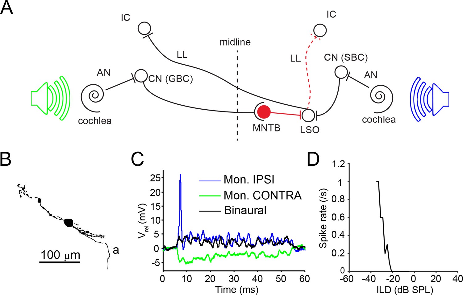
LSO circuit and basic properties.
(A) Outline of the major nuclei/cells involved in the LSO circuit. AN: auditory nerve; CN: cochlear nucleus; GBC: globular bushy cell; IC: inferior colliculus; MNTB: medial nucleus of the trapezoid body; LL: lateral lemniscus; LSO: lateral superior olive; SBC: spherical bushy cell. Speakers symbolize ipsilateral (blue) and contralateral (green) auditory stimulation. (B) Camera lucida reconstruction for a neuron with CF = 12 kHz. a: axon. (C) Example monaural ipsilateral (blue), monaural contralateral (green) and binaural (black) responses to short tones (12 kHz, 70 dB) for the neuron shown in panel B. (D) ILD function for the neuron in panel B (12 kHz, ipsilateral sound level fixed at 85 dB).
Figure 2
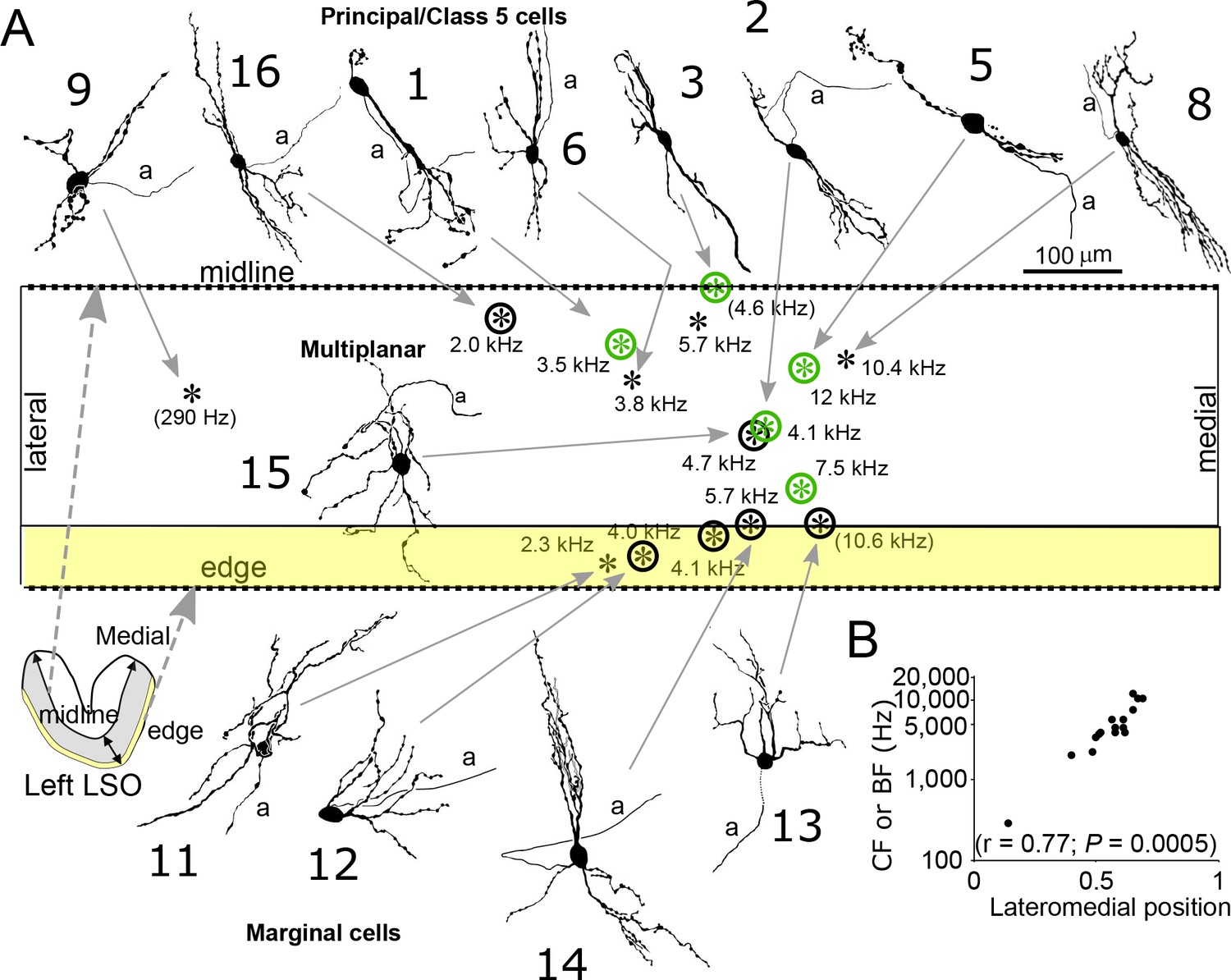
Reconstruction and location of labeled neurons.
(A) Cell body locations (asterisks) of labeled LSO neurons are shown relative to the LSO midline and edge on a flattened lateromedial map of the LSO (compare to LSO outline in the coronal plane in the lower left corner), with indication of CF or (BF). Camera lucida drawings of neurons with a well-filled dendritic tree are shown. Numbers refer to cell numbers as in Supplementary file 1. Circled asterisks represent neurons for which electron microscopic analysis was done. Green symbols indicate neurons identified as principal cells at the E.M. level. The two asterisks with no arrows pointing to them represent labeled cells with lightly labeled dendritic trees that are not illustrated. (B) CF or BF of all 15 labeled neurons as a function of normalized lateromedial cell body location (0: lateral edge; 1: medial edge).
Figure 3
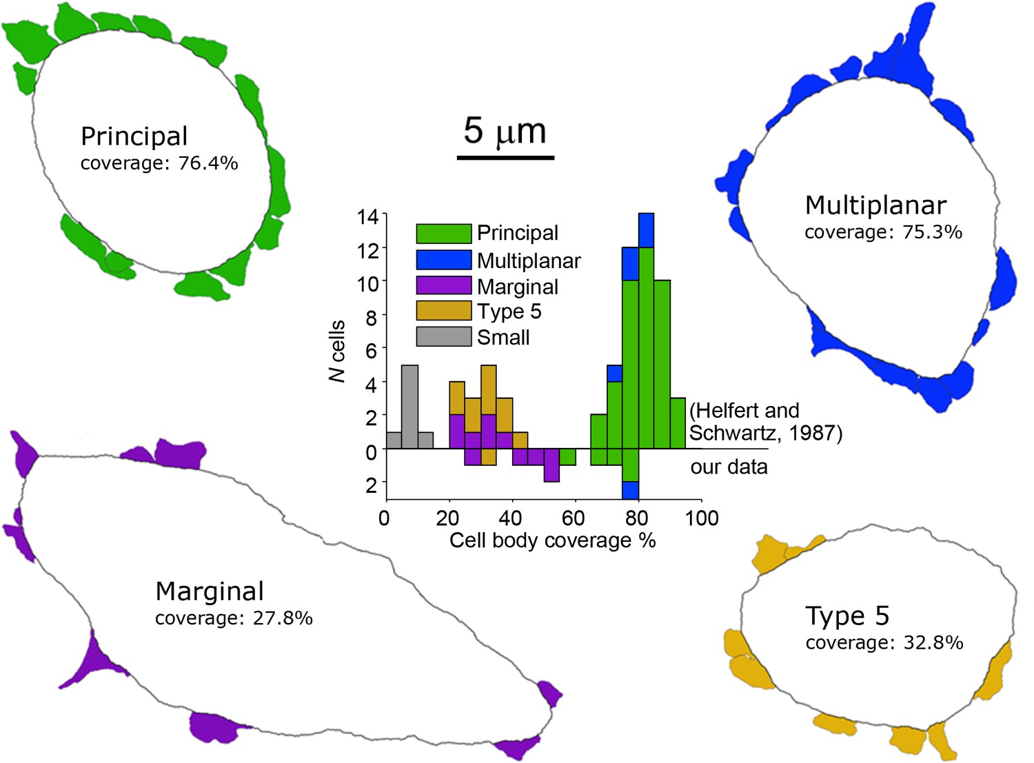
Electron microscopic analysis of cell body synaptic coverage.
Electron microscopic cell body profiles of example cells of four cell types, with colored presynaptic terminals (color coded for cell type). Middle plot shows histogram of cell body synaptic coverage for LSO cell types for the data from Helfert and Schwarz (Helfert and Schwartz, 1987) and for our data (above and below the horizontal line at 0, respectively).
Figure 4 with 1 supplement
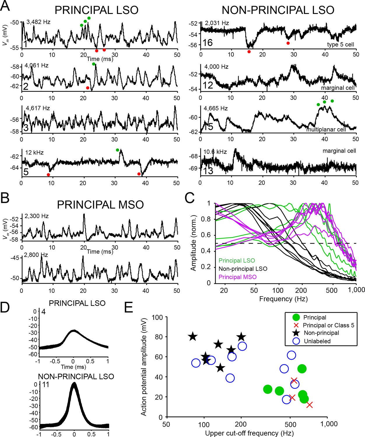
Principal cells have fast kinetics and small action potentials.
(A) Fifty milliseconds of spontaneous activity is shown for four principal cells (left column) and four non-principal cells (right column). In each panel, CF or BF is indicated (top left) as well as cell number (bottom left). For the non-principal cells in the right column, the subtype is indicated above the abscissa. Red and green dots respectively indicate examples of inhibitory and excitatory postsynaptic potentials. (B) Similar as A, for two labeled MSO neurons. (C) Normalized amplitude spectra of spontaneous activity traces for 12 LSO neurons, as well as six labeled MSO neurons (CF ranged from 2 to 3 kHz; including the examples in B). Between 2 and 6 s of spontaneous activity were analyzed for each neuron. Dashed horizontal line indicates 50% of maximal amplitude. (D) Stacked action potentials during ipsilateral sound presentations for a representative principal and a non-principal cell. Cell number is indicated in each panel. Respectively 42 (top) and 407 (bottom) action potentials are overlaid. (E) Scatter plot of average action potential amplitude versus the upper cut-off frequency. The latter was defined as the frequency where the high-frequency flank of the normalized magnitude spectrum falls to 50% of the maximal amplitude (dashed line in panel c). Green filled circles and black stars respectively indicate morphologically unambiguous principal cells and non-principal cells. Red crosses indicate labeled neurons that light microscopically could be principal cells or non-principal class 5 cells, but were not further evaluated at the E.M. level. Blue circles indicate whole-cell recordings from unlabeled LSO neurons.
Figure 4—figure supplement 1
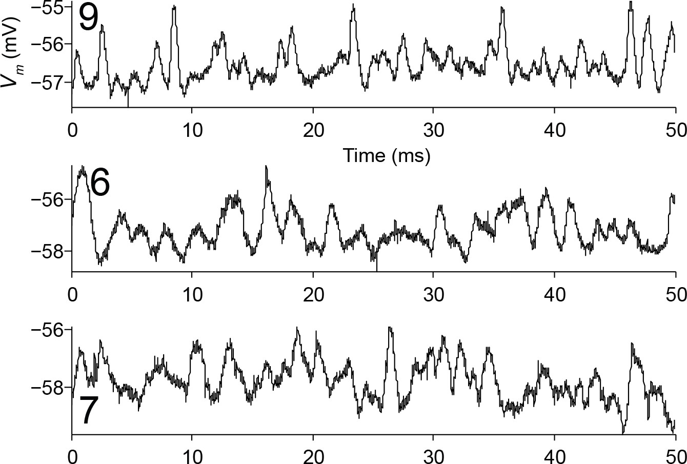
Spontaneous activity of bipolar LSO neurons.
Fifty milliseconds of spontaneous activity is shown for 3 cells that morphologically could be either principal cells or class 5 cells, but that are classified as principal based on their electrophysiology. Cell number (Supplementary file 1) is indicated in each panel.
Figure 5 with 1 supplement

Spike patterns in response to ipsilateral tones.
Dot rasters of spike responses to ipsilateral tones at or near CF or BF, for six principal cells (top) and nine non-principal cells (bottom). Each horizontal band of dots shows responses to a number of repetitions at a given SPL. CF or BF is indicated in each panel, and, for labeled cells, the cell number (Supplementary file 1).
Figure 5—figure supplement 1
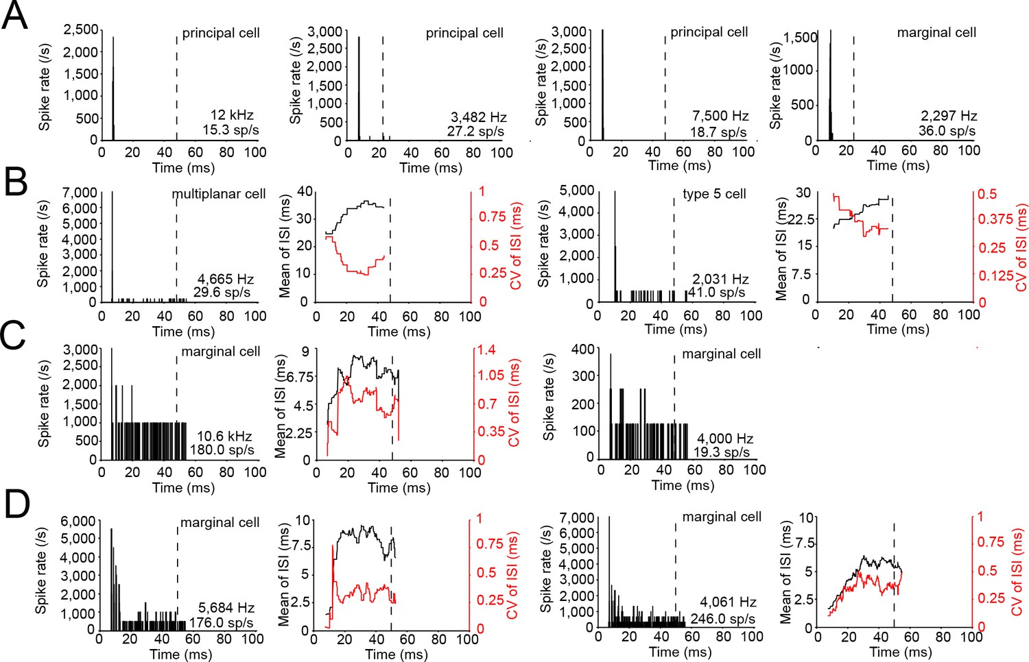
Spike patterns of labeled cells to ipsilateral tones near CF.
(A) Peristimulus time histograms (PSTH) for four cells with an onset spiking pattern. Cell type, CF and average spike rate are mentioned in each panel. Stimulus frequency/SPL for each panel/number of repetitions (from left to right): 12 kHz/70 dB SPL/30 repetitions; 3790 Hz/70 dB SPL/100 repetitions; 7500 Hz/85 dB SPL/30 repetitions; 2297 Hz/70 dB SPL/100 repetitions. Dashed vertical lines indicate stimulus duration. (B) PSTH (left panel) and mean and coefficient of variation of interspike intervals (ISI; right panel), for cells with a spiking pattern consisting of a prominent onset peak followed by low level sustained activity. Stimuli: left two panels: 4665 Hz/65 dB SPL/50 repetitions; right two panels: 2031 Hz/70 dB SPL/20 repetitions. (C) Similar to B, for two cells with a primary-like PSTH. Stimuli: left two panels: 11 kHz 75 dB SPL/10 repetitions; right two panels: 4000 Hz/90 dB SPL/80 repetitions. For the right cell, the number of spikes per trial is too low to calculate ISI statistics. (D) Similar to panel C, for two chopper cells. Stimuli: left two panels: 5684 Hz/55 dB SPL/20 repetitions; right two panels: 4061 Hz/40 dB SPL/30 repetitions. Using the criteria developed for cochlear nucleus (Young et al., 1988), these 2 LSO neurons could be classified as irregular choppers: the neuron shown in the left two panels is a chop-U unit, where the CV of ISI is highest early in the response; the neuron in the right two panels is a chop-T unit, for which the CV of ISI increases during the response and the mean ISI shows rate adaptation. Bin width is 0.1 ms for all panels.
Figure 6
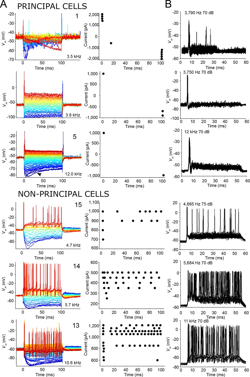
Similar spike patterns elicited by current injection and sound stimuli.
(A) Left panels: voltage responses to depolarizing and hyperpolarizing current step injection for three principal cells (top) and three non-principal cells (bottom). 0 ms corresponds to start of current injection. Colors indicate current amplitude (blue: most negative, red: most positive), and ranged respectively from (top to bottom): −2,000 to 2,000; −1,000 to 1,000; −1,000 to 1,000; −1,000 to 1,000; −500 to 500; −1,000 to 1,200 pA. The CF or BF, and cell numbers are indicated in the panel. Arrowhead (third row, left panel) indicates voltage sag indicative of Ih current that can be seen in all cell types. Right panels: spike dot rasters showing spike occurrences in the data in the left panels. (B) Stacked voltage responses to repetitions of short ipsilateral tones at or near CF/BF at one sound level, for the same cells as in A.
Figure 7 with 3 supplements
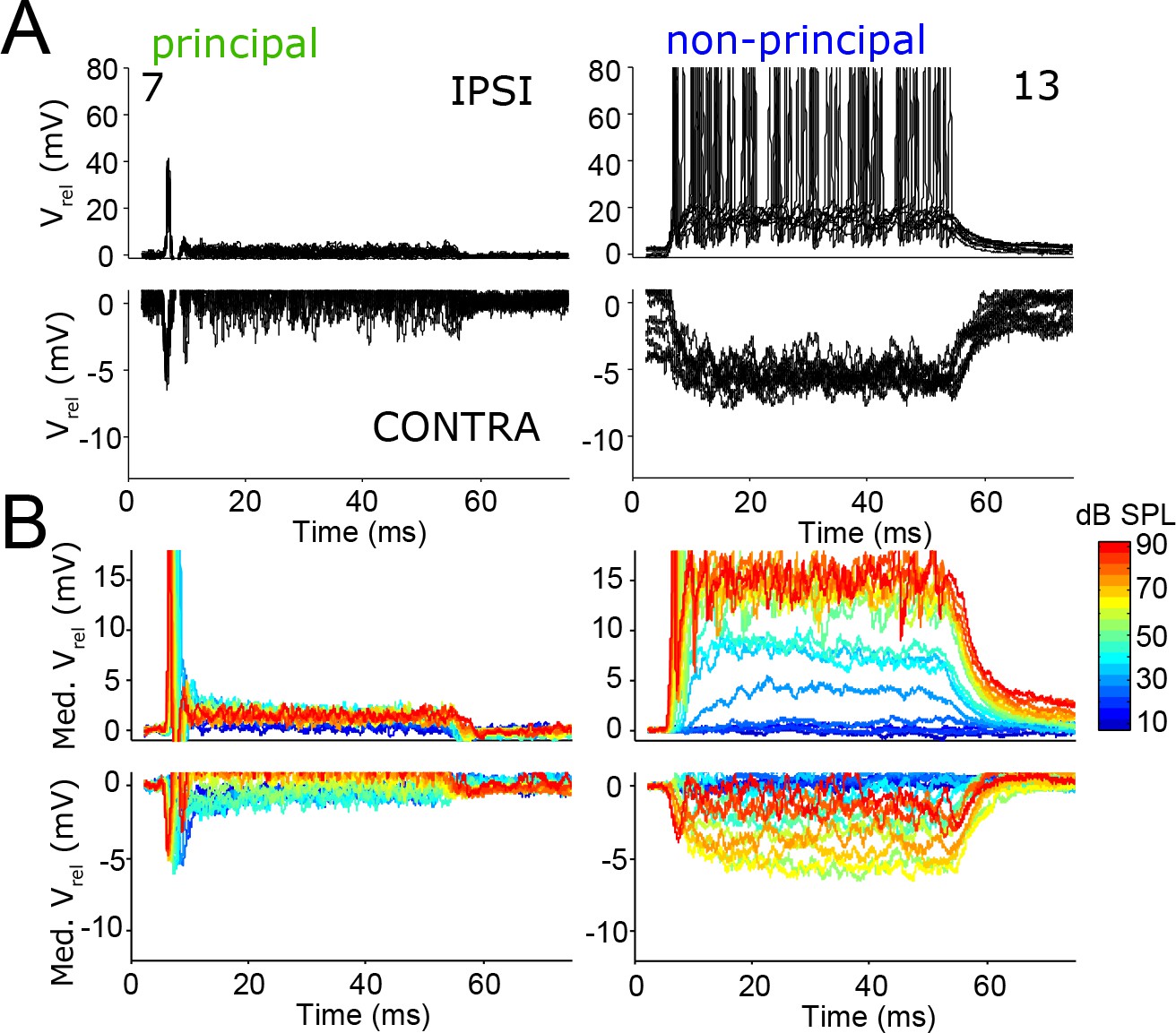
The temporal pattern of inhibition matches that of excitation.
(A) Repetitions of evoked responses to monaural ipsilateral (top panels) or contralateral (bottom panels) tones at CF or BF at 70 dB SPL, for two example neurons (numbers refer to Supplementary file 1). (B) Median Vm to ipsilateral and contralateral tones at CF or BF at different sound intensities, for the same neurons as in A. Respective stimulus frequencies and number of repetitions: 5.6 kHz, N = 20 (left column); 11 kHz, N = 10 (right column).
Figure 7—figure supplement 1

Sound-evoked excitation and inhibition is balanced.
(A) Top panel: Maximal depolarization during onset (5–15 ms post stimulus onset) for averaged responses to ipsilateral tones, as a function of sound level. Spikes occurring in or bordering intervals defined as onset (5–15 ms post stimulus onset) or sustained (40–50 ms post stimulus onset) were not included in the averages. Bottom panel: Maximal hyperpolarization during onset for averaged responses to contralateral tones, as a function of sound level. Data shown for 12 neurons. (B) Similar to A, for the sustained part of averaged subthreshold responses (40–50 ms post stimulus onset; for two neurons, 25 ms tones were used and the sustained part is calculated from 20 to 25 ms post stimulus onset). (C) Ratio of peak vs. sustained depolarization during ipsilateral tones as a function of the ratio of peak vs. sustained hyperpolarization during contralateral tones, for the same data as in A/B. Diagonal line indicates identity. (D) Maximal spike rate during ipsilateral tones versus the largest hyperpolarization during contralateral tones, for 11 neurons. Different symbols indicate different cells, where the same symbol corresponds to the same cell in each panel.
Figure 7—figure supplement 2
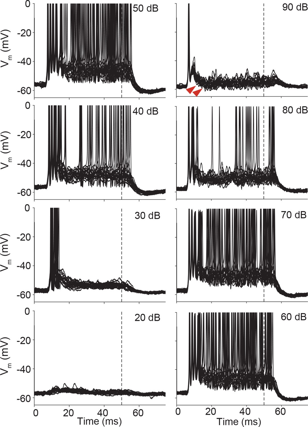
Stacked responses of a non-principal LSO cell to ipsilateral tones at CF (5.7 kHz).
At high sound intensities, IPSPs (most pronounced at 90 dB: examples indicated by red arrowheads) are evoked in addition to EPSPs and action potentials. Action potentials are clipped at 0 mV.
Figure 7—figure supplement 3
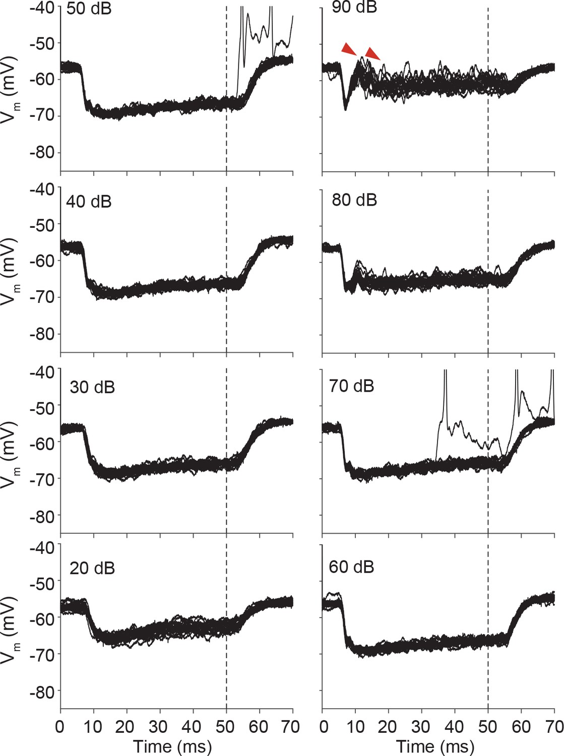
Stacked responses of the same cell as in Figure 7—figure supplement 2 to contralateral tones at CF (5.7 kHz).
At high sound intensities, EPSPs (most pronounced at 90 dB: examples indicated by red arrowheads) are evoked in addition to IPSPs.
Figure 8 with 1 supplement

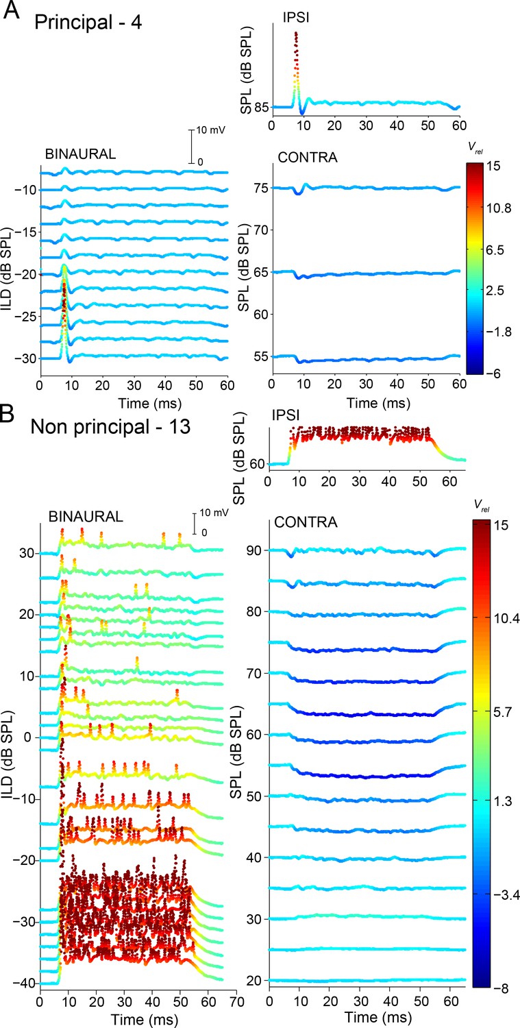
Complementary ILD-sensitivity in principal and non-principal neurons.
Average responses to binaural and monaural tones are shown for a principal cell (A) and non-principal cell (B). Average Vm is color-coded relative to resting Vm. Left panels: average responses to binaural tones of varying ILD, where the contralateral sound level is varied and the ipsilateral sound level kept constant. Right panels: average responses to monaural tones at the same sound levels as for the binaural data in the left panels. Respective stimulus frequencies: A: 3,480 Hz; B: 4,665 Hz.
Figure 8—figure supplement 1
Complementary ILD-sensitivity in principal and non-principal neurons.
Similar as Figure 8, for two other neurons. Stimulus frequencies: 7.5 kHz (A) and 11 kHz (B).
Figure 9 with 2 supplements
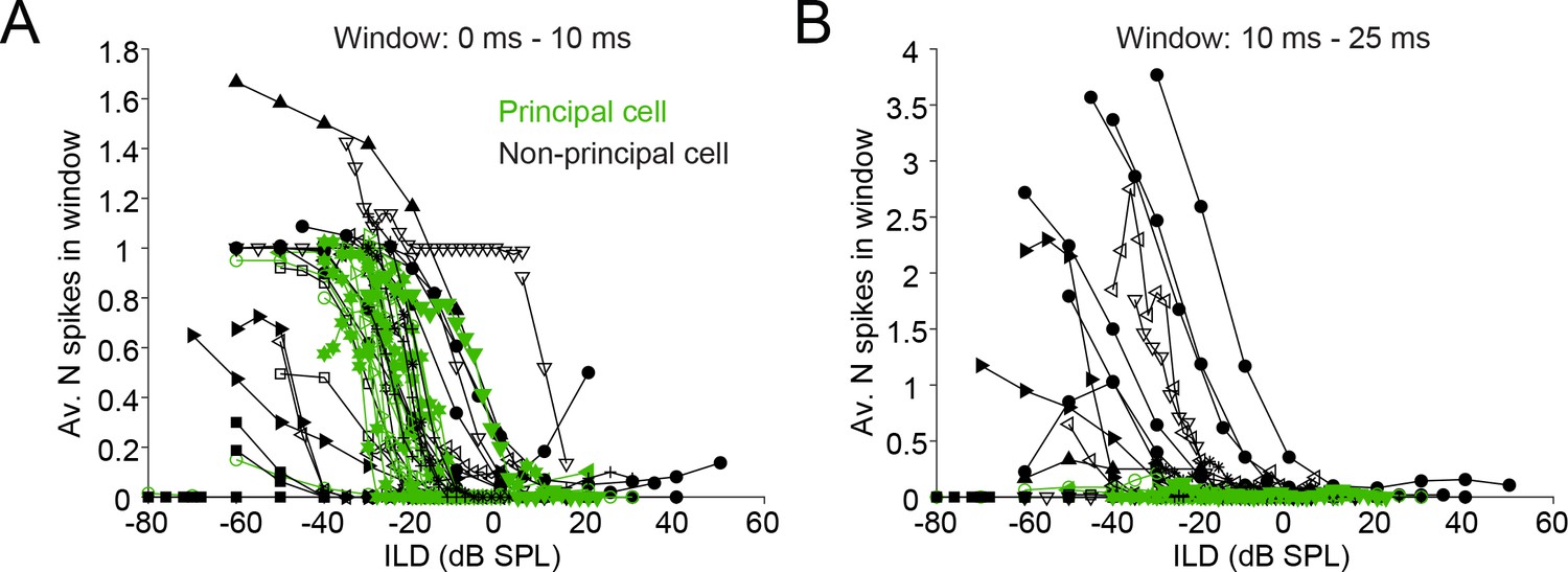
Characterization of ILD-functions in principal and non-principal neurons.
(A) ILD functions for sound onset (from 0 to 10 ms post-stimulus onset). By convention, negative (positive) values for ILD indicate a higher sound intensity at the ipsilateral (contralateral) ear. (B) ILD functions for the sustained part of the stimulus. The window is limited from 10 to 25 ms post-stimulus onset because the shortest stimulus duration used was 25 ms.
Figure 9—figure supplement 1
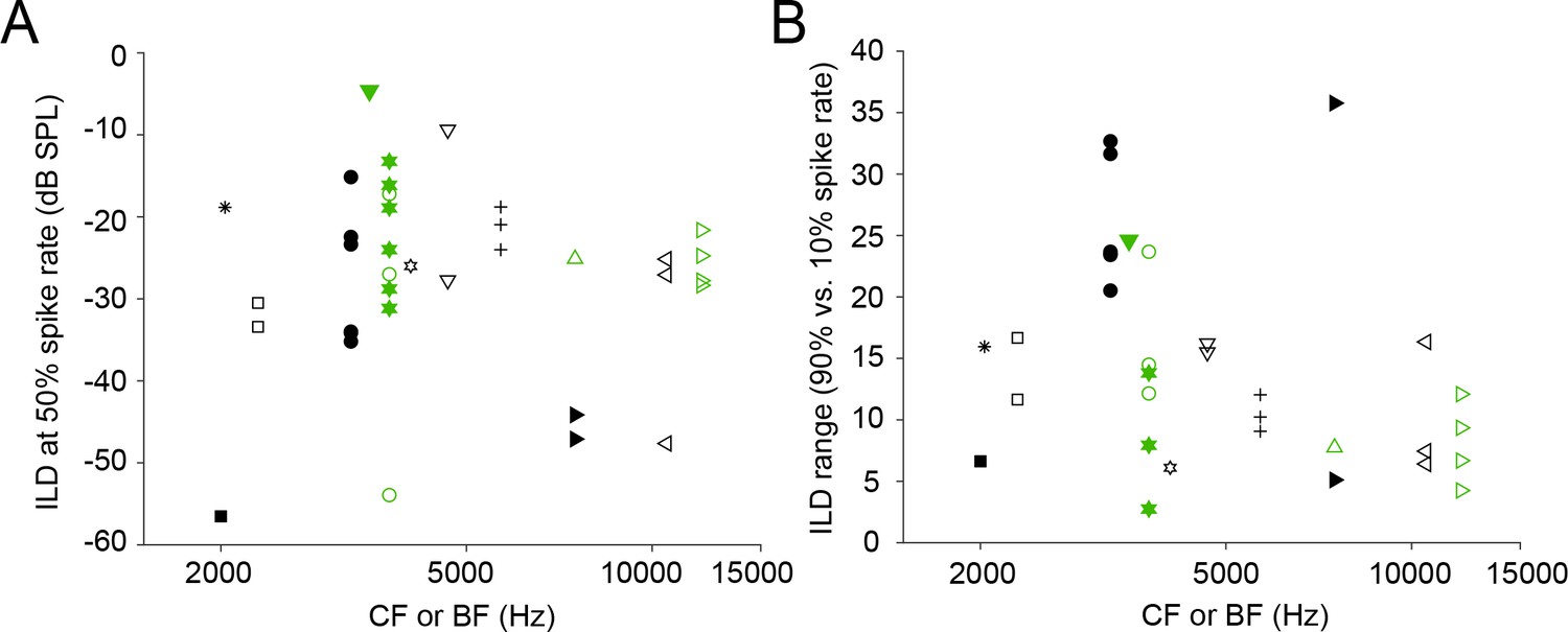
Metrics of ILD functions.
(A) ILD value at 50% spike rate for the data in Figure 9, estimated by interpolating the ILD-function using a window from 0 to 25 ms post-stimulus onset. For this analysis, only ILD functions for which the amount of data allowed us to infer the sigmoid shape and saturation level were included. (B) ILD range, defined as the difference between the ILD at 10% spike rate and the ILD at 90% spike rate, for the same data. Color code is the same in all panels. Unfilled/filled symbols indicate different neurons. Reoccurring symbols indicate separate ILD data sets, often obtained using different ipsilateral sound levels.
Figure 9—figure supplement 2
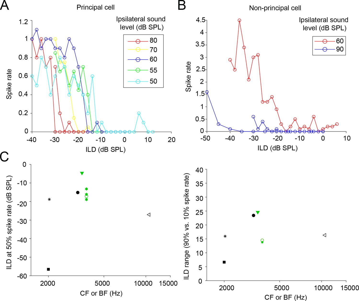
Level-dependence of ILD functions.
(A) ILD-functions of a principal cell, obtained at different ipsilateral sound levels. Spike rate is expressed as average number of spikes from 0 to 25 ms post-stimulus onset. Notice that there are two data sets with an ipsilateral sound level of 80 dB. CF: 3.8 kHz. Monaural ipsilateral threshold: 40 dB SPL. (B) Similar to A, for a non-principal cell. Notice that there are two data sets with an ipsilateral sound level of 90 dB. BF: 10.6 kHz. Monaural ipsilateral threshold: 35 dB SPL. (C) Similar to Figure 9—figure supplement 1, but now only data sets with an ipsilateral sound level lower than or equal to 25 dB above the ipsilateral monaural thresholds (similar to Sanes and Rubel, 1988) are included. This shows that for lower ipsilateral sound levels, there is a smaller number of ILD functions with 50% spiking at ILDs more negative than -20 dB SPL.
Figure 10

Collateral projections of LSO neurons.
Camera lucida drawings of 3 neurons are shown on the right: the cell number refers to the Supplementary file 1. Corresponding E.M. micrographs are shown on the left. (A) Labeled axon collateral in the LNTB from a principal LSO cell. It has large swellings suggestive of presynaptic terminals. a: axon; a.c.: axon collateral. (B,C) E.M. images of a labeled presynaptic terminal (white asterisk) from another LSO principal cell, making synaptic contact with dendritic (B) and somatic (C) compartments of an LNTB neuron. Red outline/black asterisk indicates an unlabeled large presynaptic terminal with characteristics typical of a globular bushy cell terminal. d.: dendrite; c.b.: cell body. (D,E) E.M. images of a labeled presynaptic terminal (white asterisk in D, white arrow in E) of a local axon collateral in the LSO on a cell body (c.b.). The collateral is from a non-principal multiplanar cell. Top camera lucida drawing for neuron 15 is the cell body with dendritic tree and part of the axon, bottom camera lucida drawing is the same cell body, without dendrites but with axon and axon collaterals. Arrowhead below bottom camera lucida drawing indicates the collateral whose swelling is shown in the E.M. images.
Additional files
-
Source code 1
Custom analysis scripts.legend: MATLAB code used for non-trivial analyses.
- https://doi.org/10.7554/eLife.33854.020
-
Supplementary file 1
Supplementary Table.
Overview of morphological and physiological properties of labeled LSO neurons.
- https://doi.org/10.7554/eLife.33854.021
-
Transparent reporting form
- https://doi.org/10.7554/eLife.33854.022
Download links
A two-part list of links to download the article, or parts of the article, in various formats.
Downloads (link to download the article as PDF)
Open citations (links to open the citations from this article in various online reference manager services)
Cite this article (links to download the citations from this article in formats compatible with various reference manager tools)
Principal cells of the brainstem’s interaural sound level detector are temporal differentiators rather than integrators
eLife 7:e33854.
https://doi.org/10.7554/eLife.33854


