Autistic traits, but not schizotypy, predict increased weighting of sensory information in Bayesian visual integration
- University of Edinburgh, United Kingdom
- UC Riverside, United States
Figures
Figure 1
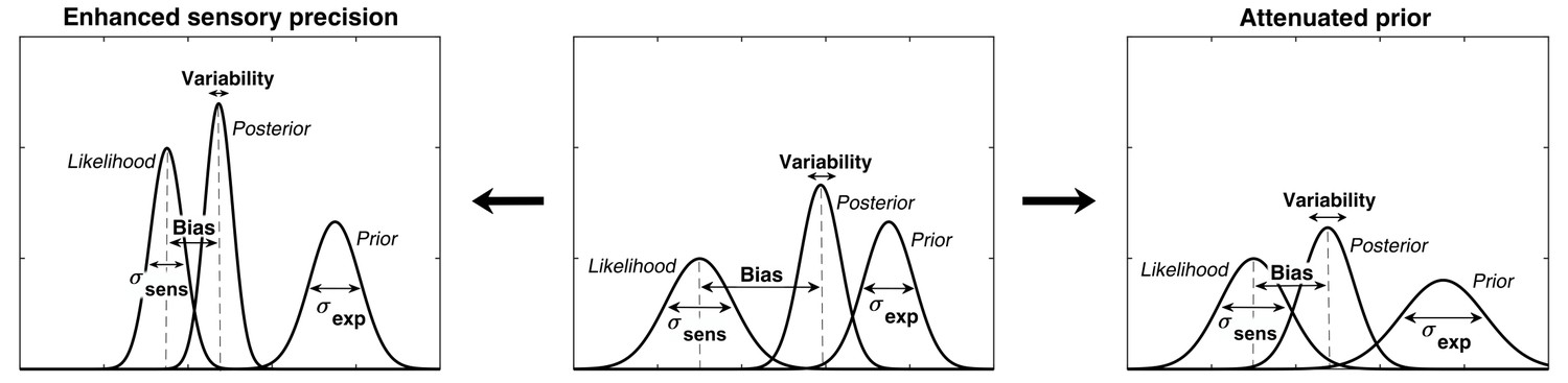
Alternative hypotheses for ASD impairments within the Bayesian inference framework.
In Bayesian terms, the percept can be described as a posterior distribution, which is a combination of sensory information (likelihood) and prior expectations (prior). Two contrasting hypotheses have been proposed to underlie behavioral differences in ASD: enhanced sensory precision, that is, smaller σsens (left) vs. attenuated priors, that is, larger σexp (right). Both hypotheses predict a reduced influence (bias) of the prior on the location of the posterior distribution (posterior mean). However, these alternatives differ in their predictions for perceptual variability, which is determined by the posterior width: the enhanced sensory precision hypothesis should lead to reduced variability while the attenuated prior hypothesis should lead to increased variability. By measuring both bias and variability, our experimental paradigm can distinguish between these two hypotheses.
Figure 2
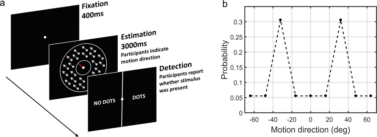
The moving dots task.
(a) Sequence of events on a single trial. First, a fixation point is presented. Next, a field of coherently moving dots is presented along with an estimation bar (extending from the fixation point) which participants are required to move to indicate perceived motion direction. Lastly, in a two-alternative forced choice, participants are asked to report whether they saw the dots during the estimation part (detection task). (b) The probability of different motion directions being presented: directions at ±32° are presented more often than other directions. Motion direction is plotted relative to a central reference angle (at 0°), which was randomly set for each participant.
Figure 3
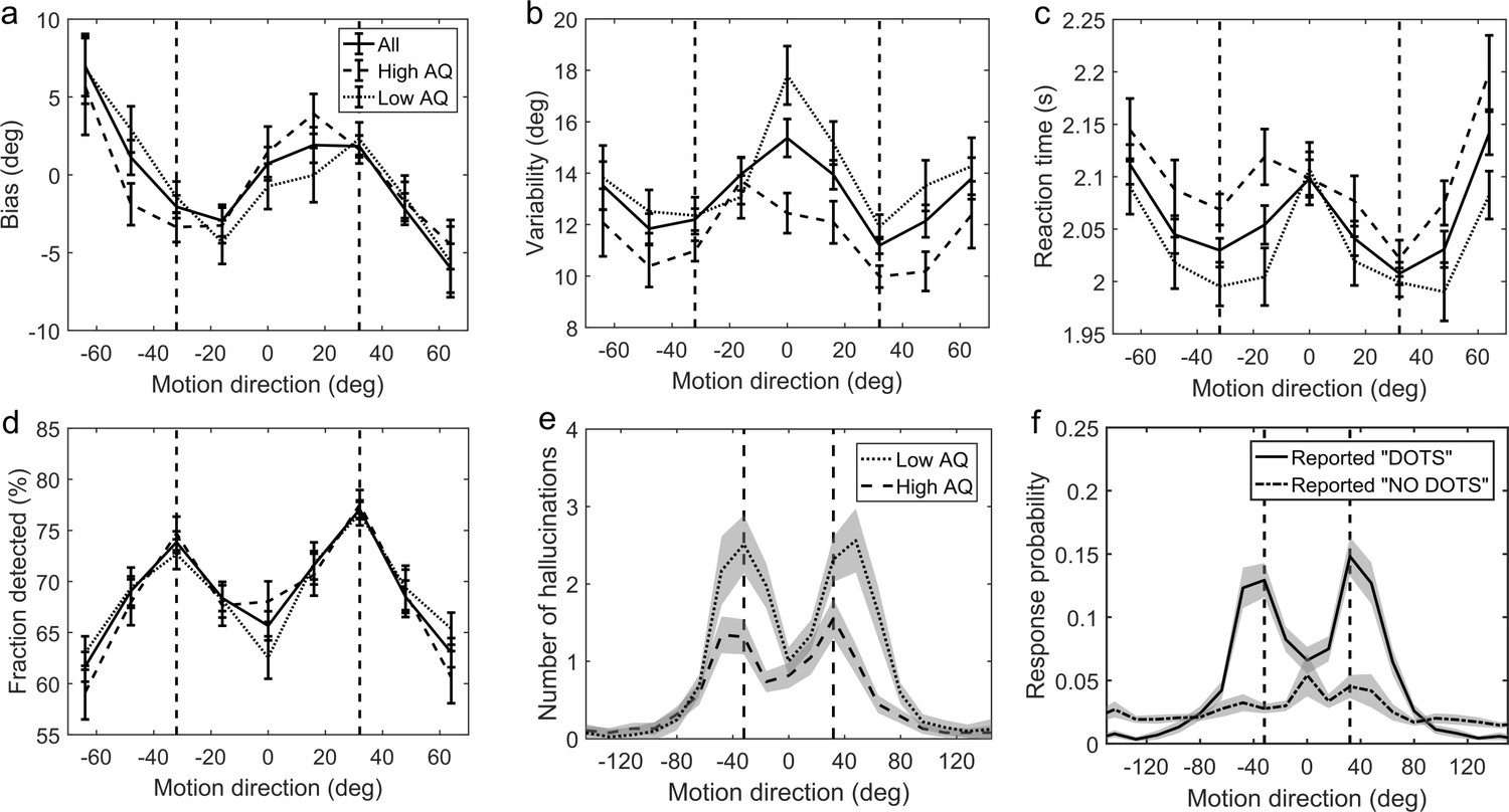
Average group performance on low-contrast trials (a–d) and on trials with no stimulus (e).
(a) Mean estimation bias, (b) standard deviation of estimations, (c) estimation reaction time and (d) fraction of trials in which the stimulus was detected. (f) Probability distribution of estimation responses on trials without stimulus. The solid line denotes the estimation responses when participants reported detecting a stimulus (hallucinations). The dash-dot line denotes estimation distributions when participants correctly reported not detecting a stimulus. (e) Distribution of hallucinations for high and low AQ groups (median split). The vertical dashed lines correspond to the two most frequently presented motion directions (±32°). Error bars and shaded areas represent within-subject standard error.
-
Figure 3—source data 1
This zip archive contains .csv files with all of the data that was used to produce plots in Figure 3.
EstimationBias.csv contains estimation biases at each of the nine presented angles. EstimationVariability.csv contains standard deviation of estimations at each of the nine presented angles. NostimDetected.csv and NostimUndetected.csv contain estimation responses when stimulus was detected and not detected, respectively, on no-stimulus trials. Traits.csv contains AQ scores of each individual (column 3) as well as all other traits. SourceData_Readme.txt contains more detailed description of each data file. The plots can be reproduced from MATLAB script master.m which is available in the provided Source code 1. SourceCode_Readme.txt contains more detailed description of the source code.
- https://doi.org/10.7554/eLife.34115.005
Figure 4
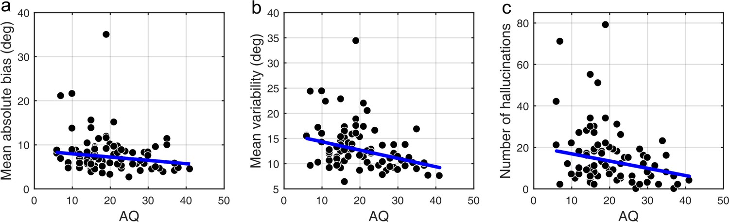
Correlations between AQ scores and task performance on low contrast trials (a, b) and when no stimulus is presented (c).
(a) Mean absolute bias (r = −0.175, p=0.053), (b) mean standard deviation (i.e. variability) of estimations (r = −0.327, p<0.001), and (c) the total number of hallucinations (r = −0.238, p=0.010). The blue lines are robust regression slopes.
-
Figure 4—source data 1
This zip archive contains .csv files with all of the data that was used to produce plots in Figure 4.
EstimationBias.csv contains estimation biases at each of the nine presented angles. EstimationVariability.csv contains standard deviation of estimations at each of the nine presented angles. NostimDetected.csv contains the number of hallucinations at different directions. Traits.csv contains AQ scores of each individual (column 3) as well as all other traits. SourceData_Readme.txt contains more detailed description of each data file. The plots were produced with MATLAB script analyze_data.m which is available in the provided Source code 1. SourceCode_Readme.txt contains more detailed description of the source code.
- https://doi.org/10.7554/eLife.34115.007
Figure 5
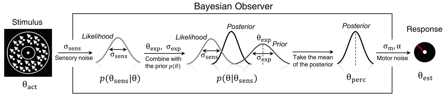
Bayesian model of estimation response for a single trial.
The actual motion direction (θact) is corrupted by sensory uncertainty (σsens), and then combined with prior expectations (mean θexp and uncertainty σexp) to form a posterior distribution. The perceptual estimate (θperc) is defined as the mean of the posterior distribution. Finally, motor precision ( ) and a probability of random response (α) are incorporated to generate the response (θest). This results in four free model parameters: σsens, σexp, θexp and α. The motor precision is estimated from high contrast trials and is used as a fixed parameter.
Figure 6
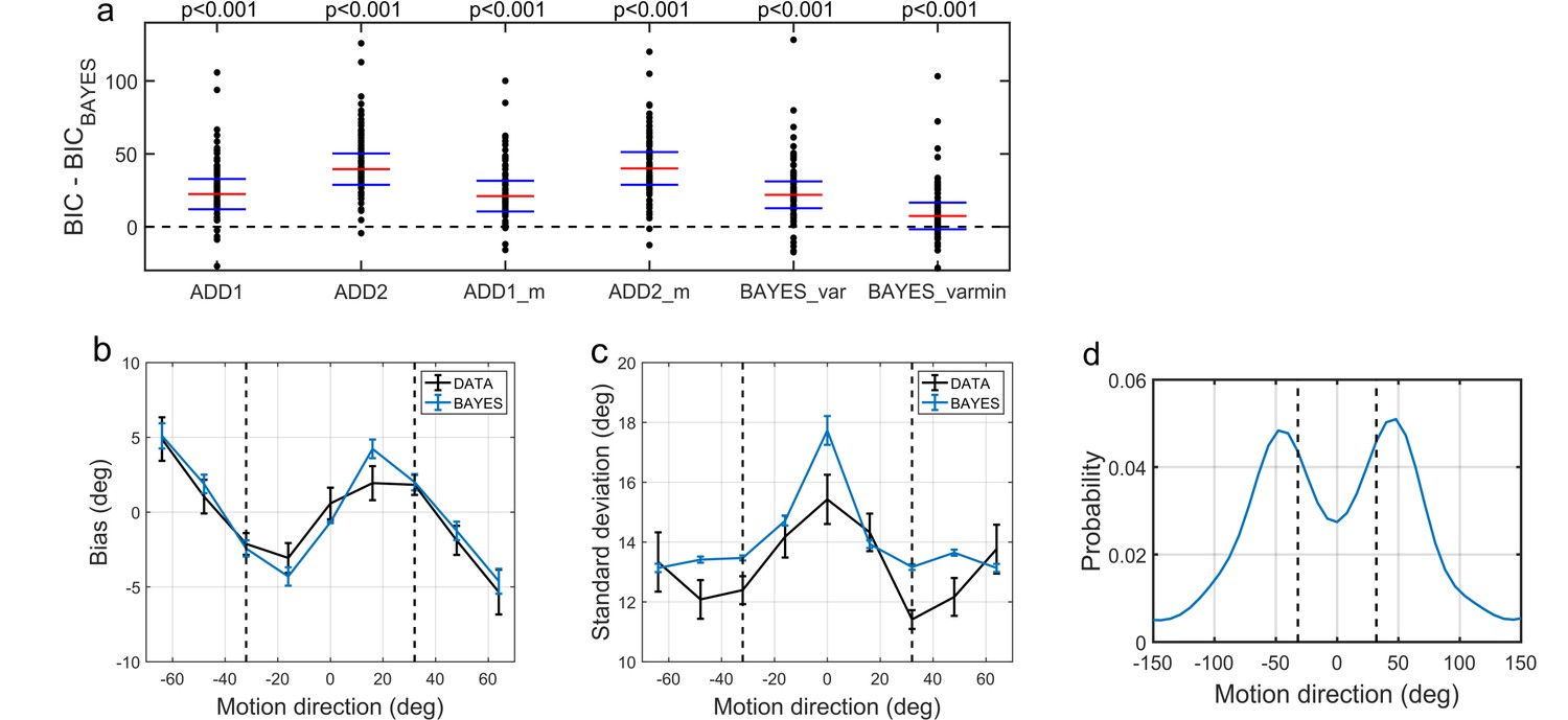
Modelling results.
(a) Model comparison for all participants using Bayesian Information Criterion (BIC). y-axis measures the relative difference between BIC of each model (as indicated on the x-axis) and BIC of BAYES model. Values greater than zero on the y-axis indicate that the BAYES model provided a better fit. Each dot represents a participant. Red horizontal lines denote median values; blue horizontal lines denote 25th and 75th percentiles. p-values above the plot indicate whether the median of the difference was significantly different from zero for each model (signed rank test). Panels (a) and (c) present task performance at different motion directions as predicted by BAYES model: (b) estimation bias, (c) standard deviation of estimations. Error bars represent within-subject standard error. (d) Population averaged prior as recovered via BAYES model. The vertical dashed lines correspond to the two most frequently presented motion directions (±32°).
Figure 7

Correlations between AQ scores and BAYES model parameters.
(a) θexp - mean of the prior expectations (r = 0.031, p=0.820), (b) σexp - uncertainty of the prior distribution (r = 0.018, p=0.962), (c) σsens - uncertainty in the sensory likelihood (r = −0.185, p=0.011) and (d) α - fraction of random estimations (r = −0.135, p=0.238). The blue lines are robust regression slopes.
-
Figure 7—source data 1
This zip archive contains .csv files with all of the data that was used to produce plots in Figure 7.
BayesEstimatedParams.csv contains BAYES model parameter estimates. Traits.csv contains AQ scores of each individual (column 3) as well as all other traits. SourceData_Readme.txt contains more detailed description of each data file. The plots were produced with MATLAB script analyze_params.m which is available in the provided Source code 1. The SourceCode_Readme.txt contains more detailed description of the source code.
- https://doi.org/10.7554/eLife.34115.011
Figure 8
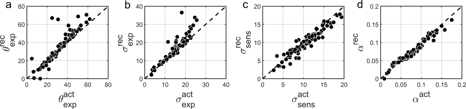
Comparison of actual (x-axis) vs. recovered (y-axis) parameters using the BAYES’ model.
(a) θexp - mean of the prior expectations (r = 0.90), (b) σexp - uncertainty of the prior distribution (r = 0.92), (c) σsens - uncertainty in the sensory likelihood (r = 0.95), (d) α - fraction of random estimations (r = 0.98). The dashed diagonal line is a reference line indicating perfect parameter recovery.
Appendix 1—figure 1

Task performance at the highest contrast level and exclusion Criteria.
Left panel: fraction of detected high contrast trials - quantified as the fraction of trials in which participants both validated their choice with a click within 3000 ms in the estimation part and reported seeing dots (clicked ‘DOTS’) in the detection part. Right panel: root mean square error of estimations on high contrast trials. The dashed lines represent minimum performance criteria (more than 80% detection and less than 30° RMS error of estimations). Excluded participants are denoted by cross markers.
Appendix 1—figure 2
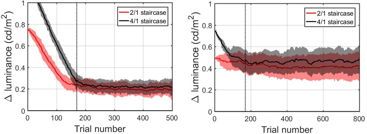
Population averaged stimulus contrast relative to the background contrast for the 2/1 (red) and 4/1 (black) staircased contrast levels.
Standard deviation is denoted by shaded areas with corresponding colors. The vertical dashed line marks 170 trials. Left panel: 44 participants (remaining after exclusion) that performed the task with the background luminance set to 1.16 cd/m2. Right panel: 39 participants (remaining after exclusion) that performed the task with the background luminance set to 5.18 cd/m2.
Appendix 1—figure 3

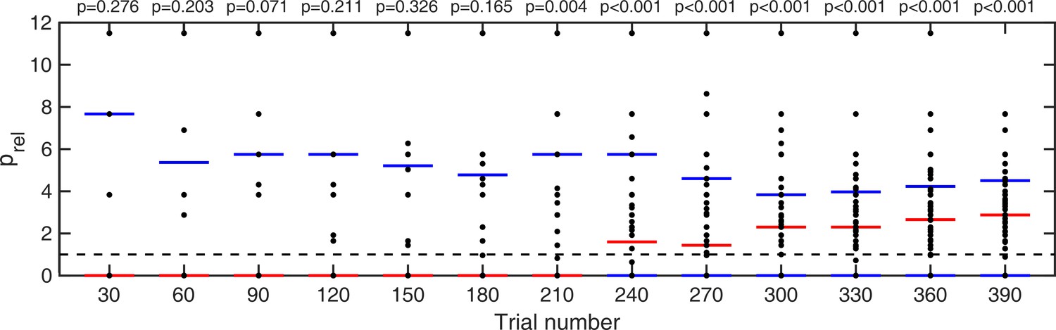
Cumulative moving average of ratio of estimation reaction times at ±32° vs average reaction times at all other directions.
Red bars indicate median values and blue bars indicate 25th and 75th percentiles. p-values indicate whether RTs at ±32° are significantly shorter than average RTs over all other directions (one-tailed Wilcoxon signed rank test).
Appendix 1—figure 4
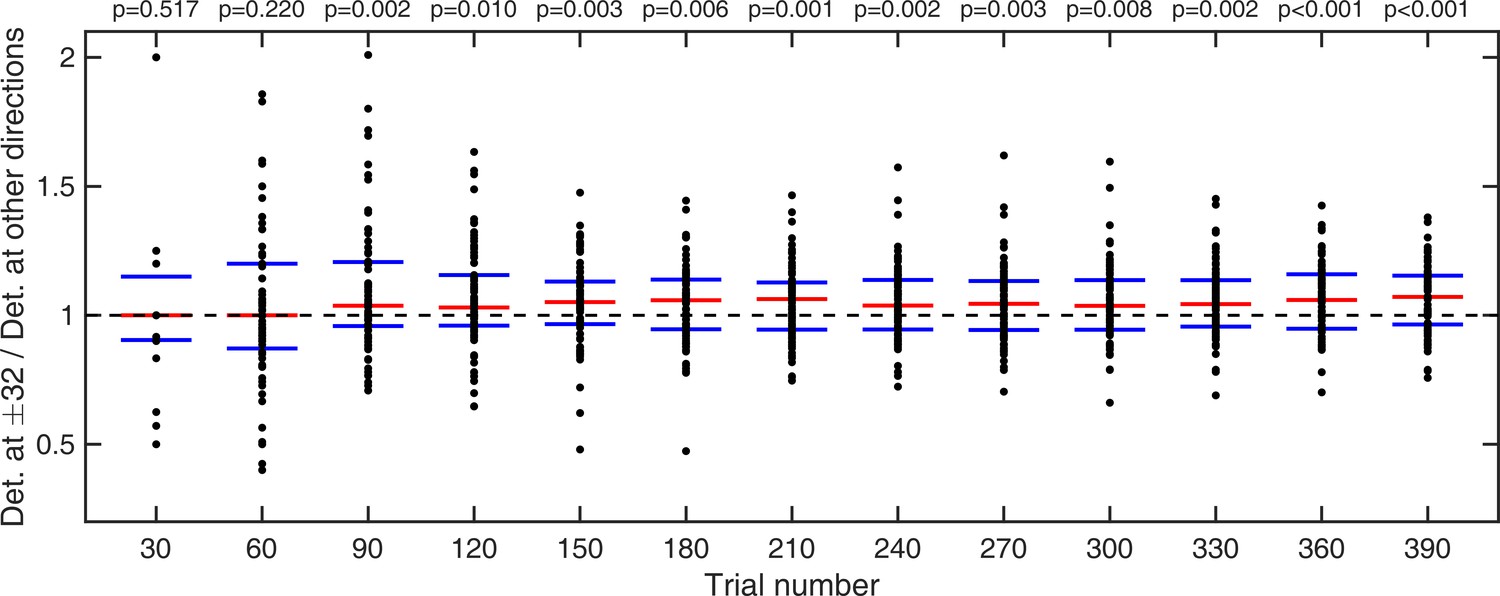
Cumulative moving average of ratio of fraction of detected stimuli at ±32° vs average fraction detected at all other directions.
Red bars indicate median values and blue bars indicate 25th and 75th percentiles. p-values indicate whether fraction detected at ±32° are significantly larger than average fraction detected over all other directions (one-tailed Wilcoxon signed rank test).
Appendix 1—figure 5
Cumulative moving average of ratio of fraction of detected stimuli at ±32° vs average fraction detected at all other directions.
Red bars indicate median values and blue bars indicate 25th and 75th percentiles. p-values indicate whether fraction detected at ±32° are significantly larger than average fraction detected over all other directions (one-tailed Wilcoxon signed rank test).
Appendix 1—figure 6
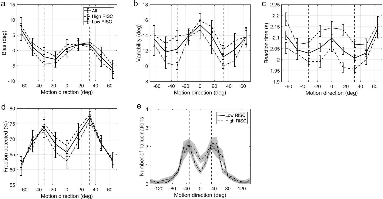
Average group performance on low-contrast trials (a–d) and on trials with no stimulus (e) by groups split by median RISC score.
(a) Mean estimation bias, (b) standard deviation of estimations, (c) estimation reaction time and (d) fraction of trials in which the stimulus was detected. (e) Distribution of hallucinations. The vertical dashed lines correspond to the two most frequently presented motion directions (±32°). Error bars and shaded areas represent within-subject standard error.
Appendix 1—figure 7
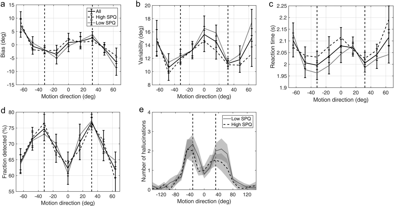
Average group performance on low-contrast trials (a–d) and on trials with no stimulus (e) by groups split by median SPQ score.
(a) Mean estimation bias, (b) standard deviation of estimations, (c) estimation reaction time and (d) fraction of trials in which the stimulus was detected. (e) Distribution of hallucinations. The vertical dashed lines correspond to the two most frequently presented motion directions (±32°). Error bars and shaded areas represent within-subject standard error.
Appendix 1—figure 8
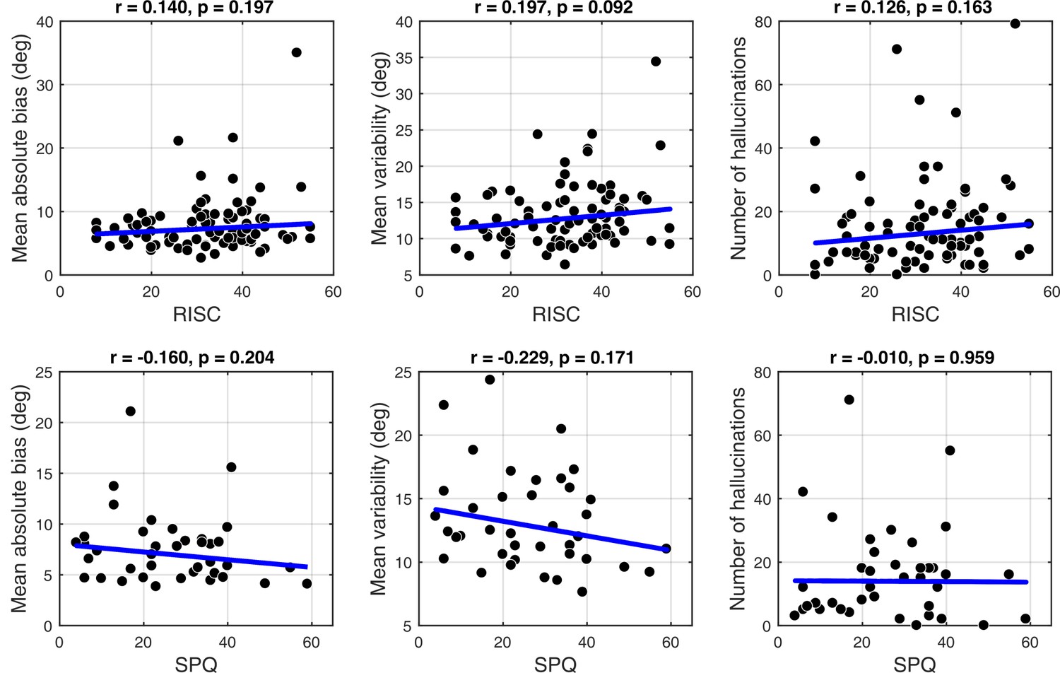
Correlations between personality traits, RISC (top row) and SPQ (bottom row) and task performance.
There were no significant correlations with any of the measures: mean absolute bias (left column), mean estimation variability (middle column) and total number of hallucinations (right column). Robust correlation coefficients and p-values are indicated above each plot. The blue lines denote robust regression.
Appendix 1—figure 9

Correlations with the BAYES model parameter values and schizotypy traits (as measured by both RISC and SPQ).
First column: θexp - mean of the prior expectations, second column: σexp - uncertainty of the prior distribution, third column: σsens - uncertainty in the sensory likelihood and fourth column: α - fraction of random estimations. Robust correlation coefficients and p-values are indicated above each plot. The blue lines denote robust regression.
Appendix 1—figure 10
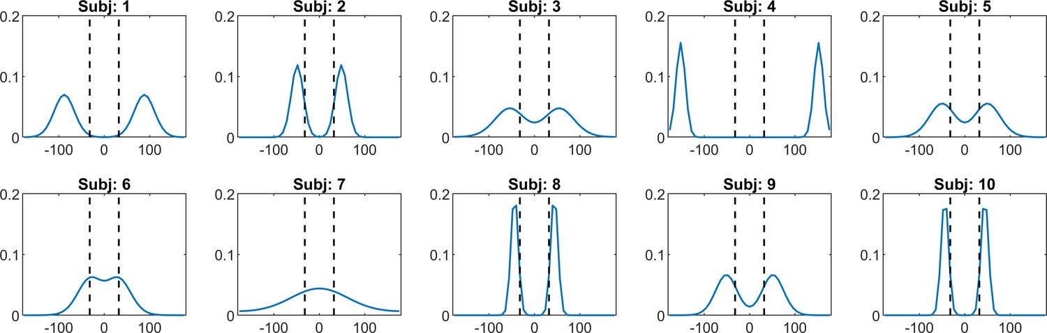
A representative sample of prior expectations for each individual as reconstructed via ‘BAYES’ model.
The dashed lines correspond to the two most frequently presented motion directions (±32°).
Appendix 2—figure 1
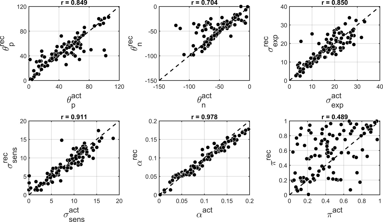
Comparison of actual and recovered parameters via ‘BAYES_π’ model.
θp and θn - positive and negative modes of the bimodal distribution of prior expectations, σexp - uncertainty of the prior distribution, σsens uncertainty in the sensory likelihood, α - fraction of random estimations, π - mixing parameter responsible for the degree of bimodality. Actual parameters are scattered along x-axis and recovered parameters are scattered along y-axis. The dashed diagonal line is a reference line indicating perfect parameter recovery. Pearson’s correlation coefficients are indicated above each plot.
Appendix 2—figure 2
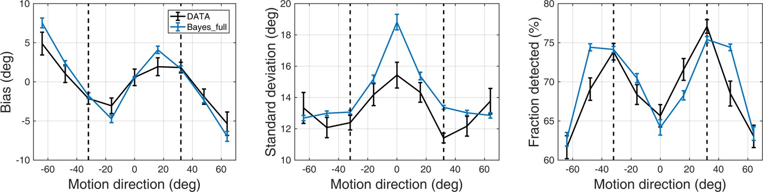
Task performance as predicted by the BAYES_full model.
Left panel: mean estimation bias at different motion directions. Middle panel: standard deviation of estimations at different motion directions. Right panel: fraction of detected stimuli at different motion directions. The dashed lines correspond to the two most frequently presented motion directions (±32°). Error bars represent within-subject standard error.
Appendix 2—figure 3
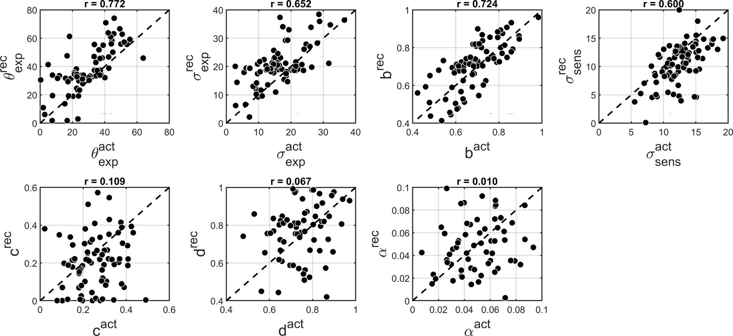
Comparison of actual and recovered parameters via ‘BAYES_full’ model.
θexp - the mean of prior expectations of motion direction, σexp - uncertainty of the prior expectations of motion direction, σsens - uncertainty in the sensory likelihood, α - fraction of random estimations, b - prior expectation for dots being presented, c likelihood of detecting the dots when they are not presented, d - likelihood of detecting the dots when they are presented. Actual parameters are scattered along x-axis and recovered parameters are scattered along y-axis. The dashed diagonal line is a reference line indicating perfect parameter recovery.
Additional files
-
Source code 1
Matlab scripts for data analysis and reproduction of the figures presented in the article.
- https://doi.org/10.7554/eLife.34115.013
-
Transparent reporting form
- https://doi.org/10.7554/eLife.34115.014
Download links
A two-part list of links to download the article, or parts of the article, in various formats.
Downloads (link to download the article as PDF)
Open citations (links to open the citations from this article in various online reference manager services)
Cite this article (links to download the citations from this article in formats compatible with various reference manager tools)
Autistic traits, but not schizotypy, predict increased weighting of sensory information in Bayesian visual integration
eLife 7:e34115.
https://doi.org/10.7554/eLife.34115


