Recurrent network model for learning goal-directed sequences through reverse replay
Figures
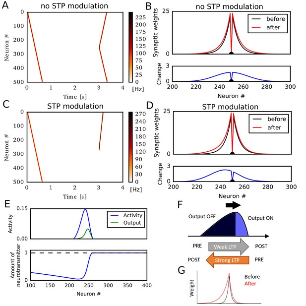
Potentiation of reverse propagation in 1-D recurrent network of rate neurons.
(A, C) Weight modifications were induced by a firing sequence in a 1-D recurrent network (at time 0 s), and the effects of these changes on sequence propagation were examined at time 3 s. Recurrent synaptic weights were modified by the standard Hebbian plasticity rule (A) or the revised Hebbian plasticity rule, where the latter was modulated by STP. (B, D) Weights of outgoing synapses from neuron #250 to other neurons are shown at time 0 s (black) and 3 s (red) of the simulations in (A) and (C), respectively (top). Lower panels show the weight changes (blue). (E) Neural activity, presynaptic outputs (top) and the amount of neurotransmitters at presynaptic terminals (bottom) are shown at 300 ms of the simulation in (C). (F) Activity packet traveling on the 1-D recurrent network and the resultant weight changes by the revised Hebbian plasticity rule are schematically illustrated. (G) Distributions of synaptic weights are schematically shown before and after a sequence propagation.
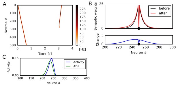
Potentiation of reverse propagation in 1-D recurrent network with accumulation of afterdepolarization (ADP).
In this simulation, we show that ADP can generate direction-selective synaptic potentiation similar to those for STP. Here, Hebbian plasticity is modulated by ADP, but not by STP (Experimental Procedure). (A) Weight modifications were induced by a firing sequence in a 1-D recurrent network (at time 0 s), and the effects of these changes on sequence propagation were examined at time 3 s. Recurrent synaptic weights were modified by the revised Hebbian plasticity rule in which the contribution of postsynaptic activities were determined by ADP accumulated through time. (B) Weights of outgoing synapses from neuron #250 to other neurons are shown at time 0 s (black) and 3 s (red) of the simulations in (A) (top). Lower panels show the weight changes (blue). (C) Neural activity and accumulated effects of ADP are shown at 300 ms of the simulation in (A).
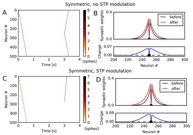
Potentiation of reverse propagation in 1-D recurrent network of spiking neurons.
(A, C) Simulations similar to those shown in Figure 1 were performed in a 1-D spiking neural network. Recurrent synaptic weights were changed by symmetric STDP. In (A) the plasticity rules were not modulated by STP whereas in (C) the rules were modulated. (B, D) The weights of outgoing synapses from neuron #250 (top) are shown at time 0 s (black) and 3 s (red) of the simulation settings shown in (A) and (C), respectively. Lower panels display the weight changes (blue).
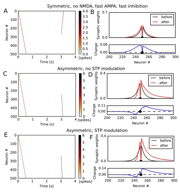
Simulation of 1-D spiking neural network in various conditions.
(A,C,E) Simulations similar to those shown in Figure 1 were performed in a 1-D spiking neural network. Recurrent synaptic weights were changed by symmetric STDP (A) or asymmetric STDP (C,E). In (C), the plasticity rules were not modulated by STP whereas in (A) and (E) the rules were modulated. In (A), we turned off NMDA current, and time constants of AMPA and inhibition were half of other simulations. (B,D,F) The weights of outgoing synapses from neuron #250 (top) are shown at time 0 s (black) and 3 s (red) of the simulation settings shown in (A), (C), and (E), respectively. Lower panels display the weight changes (blue).
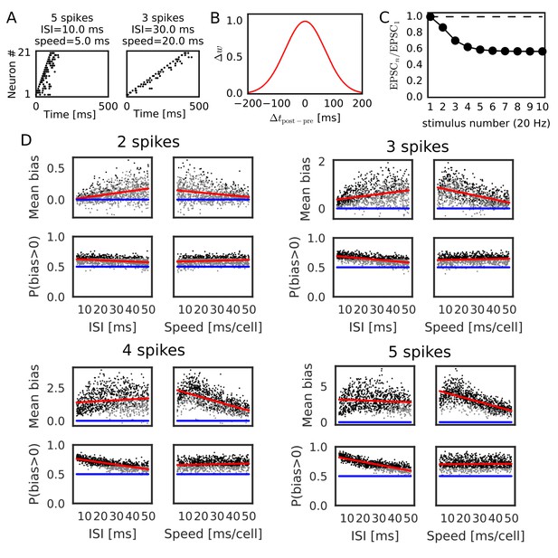
Reversely biased weight changes for symmetric STDP against variations in firing patterns.
(A) Two examples show firing sequences having different ISIs and propagation speeds. (B) Gaussian-shaped symmetric STDP was used in the simulations (c.f., Figure 1 in Mishra et al., 2016). (C) Changes in the amplitude ratio of EPSC during a 20 Hz stimulation are shown (c.f., Supplementary Figure 5 in Guzman et al., 2016). See the text for the parameter setting. (D) The mean (top) and fraction (bottom) of biases towards reverse direction are plotted for various parameter settings. A more positive bias indicates stronger weight changes in the reverse direction. Black dots correspond to parameter settings giving statistically significant positive or negative biases (p<0.01 in Wilcoxon signed rank test for the mean bias or binomial test for P(bias >0)), whereas grey dots are not significant. Red lines are linear fits to the data and blue lines indicate zero-bias (mean bias = 0 and P(bias >0)=0.5). See also Table 1.

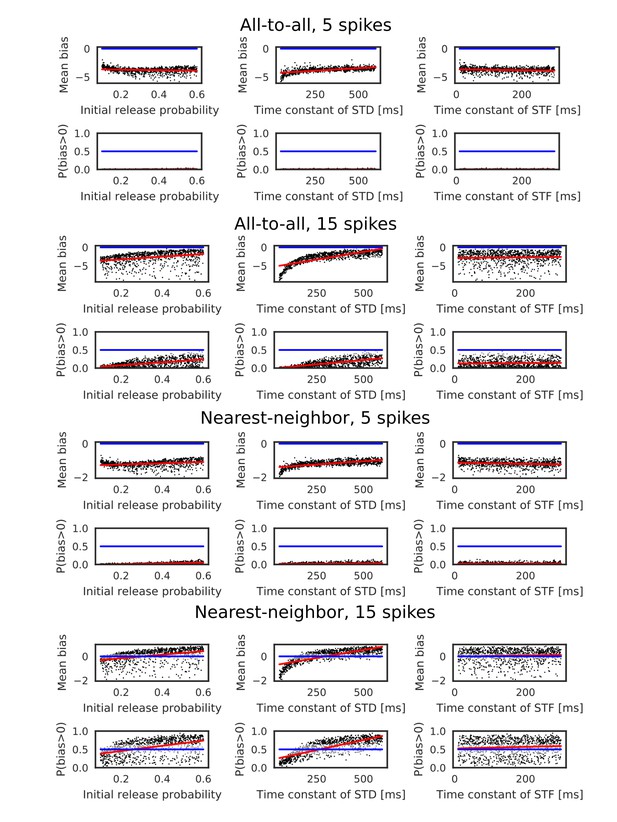
Reversely biased weight changes against variations in short-term plasticity.
The mean and fraction of positive biases toward reverse direction are shown in various parameter settings of short-term plasticity, where a more positive bias indicates stronger weight changes in the reverse direction. Black dots correspond to parameter settings giving statistically significant positive or negative biases (p<0.01 in Wilcoxon signed rank test for the mean bias or binomial test for P(bias >0)), whereas grey dots are not significant. Red lines are linear fits to the data and blue lines indicate zero-bias (mean bias = 0 and P(bias >0)=0.5). See also Table 1.
Evaluation of biases toward reverse direction for asymmetric STDP.
The mean and fraction of positive biases toward reverse direction are shown in various parameter settings of short-term plasticity, where a more positive bias indicates stronger weight changes in the reverse direction. Black dots correspond to parameter settings giving statistically significant positive or negative biases (p<0.01 in Wilcoxon signed rank test for the mean bias or binomial test for P(bias >0)), whereas grey dots are not significant. Red lines are linear fits to the data and blue lines indicate zero-bias (mean bias = 0 and P(bias >0)=0.5).
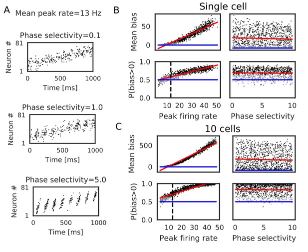
Bias effects induced by place-cell activity during run.
Simulations similar to those in Figure 3 were performed with spike trains mimicking theta sequences of place-cell firing during run. (A) Examples of spike trains in simulations of place-cell activity during run. We had two tuning parameters: mean peak firing rate and phase selectivity. The latter controls theta-phase locking of spikes. (B) The mean and fraction of positive biases to the reverse direction calculated from a single central neuron are shown in various parameter settings. A more positive bias indicates stronger weight changes in the reverse direction. Black dots correspond to the parameter settings yielding statistically significant positive or negative biases (p<0.01 in Wilcoxon signed rank test for the mean bias or binomial test for P(bias >0)), whereas grey dots are not significant. Red lines are linear fits to the data and blue lines indicate zero-bias (mean bias = 0 and P(bias >0)=0.5). (C) Same as B, but biases were summed over 10 neurons at the center. In B and C, the width of the STDP time window was 70 ms. See also Table 2.
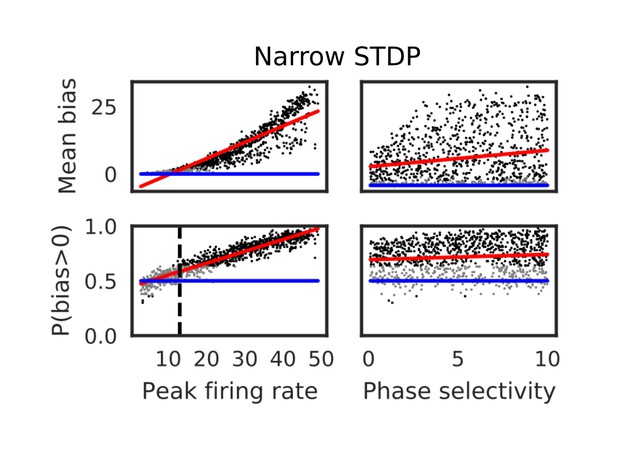
Bias effects during run induced by narrowed symmetric STDP.
Here, the STDP time window was narrowed to =10 ms. The mean and fraction of positive biases toward the reverse direction were calculated from a single central neuron in various parameter settings. A more positive bias indicates stronger weight changes in the reverse direction. Black dots correspond to parameter settings giving statistically significant positive or negative biases (p<0.01 in Wilcoxon signed rank test for the mean bias or binomial test for P(bias>0)), whereas grey dots are not significant. Red lines are linear fits to the data and blue lines indicate zero-bias (mean bias=0 and P(bias>0)=0.5). See also Table 2.
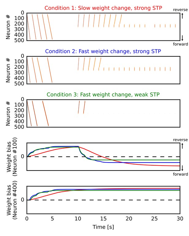
Learning a forward synaptic pathway through reverse replay.
We induced forward firing sequences in the 1-D recurrent network from 0 s to 5 s, and then stimulated neurons at the center from 10 s to 30 s. We simulated three conditions in which parameters for long-term and short-term plasticity were different (see the main text). (A, B, C) Simulated neural activities in conditions 1, 2 and 3, respectively. We used a long time constant for long-term plasticity and strong short-term depression in the condition 1. Compared with the condition 1, the time constant was shortened in the condition 2 and short-term depression was also weakened in the condition 3. (D, E) Changes in the directional biases of synaptic weights on neurons #100 and #400, respectively. Red, blue and green lines correspond to the conditions 1, 2 and 3, respectively. A more positive bias indicates stronger weights in the reverse direction of the initial forward sequences.
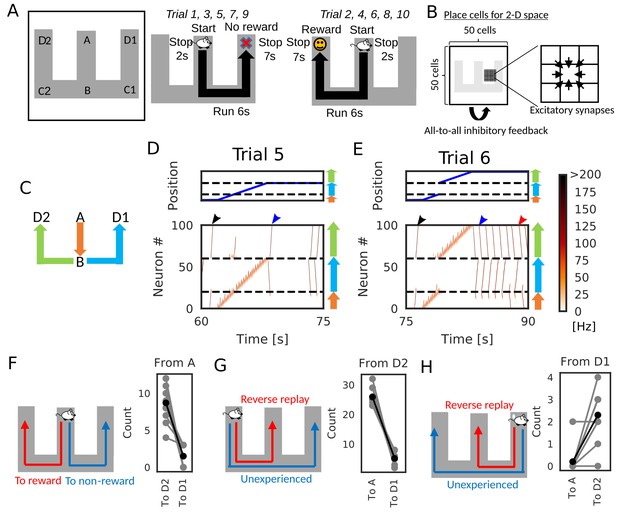
Goal-directed path learning with reverse replay on a W-maze.
(A) An animal alternately repeats traverses from starting position A to two goal positions D1 and D2 on a track. (B) Schematic illustration of a 2-D recurrent network of place cells. The conjunction of receptive fields of all place cells covers the entire track. Adjacent place cells were interconnected via excitatory synapses. (C) A color code specifies the three portions of the W-maze in the following linearized plots. (D, E) Linearized plots of the animal’s position (top) and simulated neural activities of place cells on the track (bottom). Black arrows indicate the end points of goal-directed sequences from A to D2 through B, a red arrow indicates the starting points of reverse replay from D2 to A through B, and blue arrows indicate the end point and starting point of replays through unexperienced paths D1 to D2 (trial 5) and D2 to D1 (trial 6), respectively. (F, G, H) The number of firing sequences triggered from A (F), from D2 (G) and from D1 (H) in each of 10 independent simulation sets (gray points). Black points show the means taken over the simulation sets.
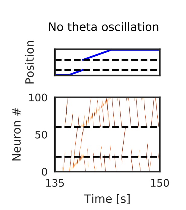
Simulated place-cell activity without theta oscillation on W-maze.
Typical neural activities on the W-maze when we turned off theta oscillation. Firing sequences propagated long distances to both forward and reverse directions even during run.
Simulation of goal-directed path learning with reverse replay in a 2-D recurrent neural network.
Movie of neural activities in the simulations shown in Figure 7. The pseudo-color map corresponds to the firing rates (Hz) of place cells arranged on a 2-D square lattice. Firing rates above 200 Hz was truncated to 200 Hz. White circle shows the current position of the animal.
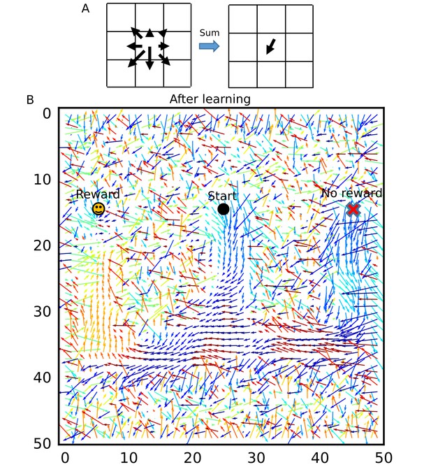
Recurrent connections organized on the W-maze for activity propagation toward reward.
(A) Calculation of connection vectors at each position on the W-maze is schematically illustrated. Vector length in the left figure corresponds to synaptic weights. (B) The connection vectors formed through reverse replay point the directions leading to the rewarded goal along the track. Note that these vectors are meaningful only inside of the maze because the outside positions were not visited by the animal and the corresponding vectors merely represent the untrained initial states.
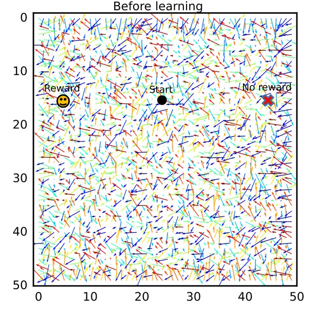
The connection vector field before exploration on the W-maze.
Connection vectors were calculated from the initial synaptic weights. Connection vectors pointed random directions.
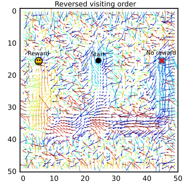
The connection vector field after exploration in a different order.
The connection vector field after learning was calculated for a simulation setting in which the two arms were alternately visited in an order different from that of the simulation setting in Figure 7. Essentially the same results were obtained.
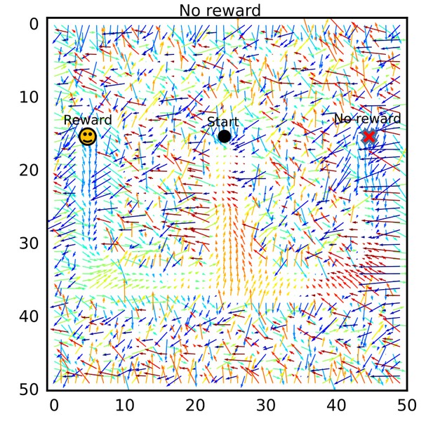
The connection vector field after learning without reward.
The connection vector field after learning was calculated for a simulation setting in which no reward (no dopamine signal) was given. The vector field shows flows from the goal positions to the start position.
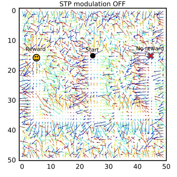
The connection vector field after learning without modulation by short-term plasticity.
The connection vector field after learning was calculated for a simulation setting in which long-term plasticity was not modulated by short-term plasticity (STP). No consistent flows were formed.
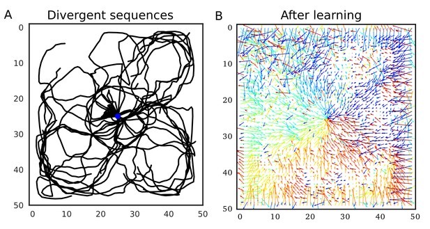
Divergent firing sequences create convergent weight biases to the triggering point.
(A) Trajectories of divergent firing sequences triggered at the center (blue circle) in a 2-D neural network. We plotted positions of the gravity center of instantaneous neural activities during sequence propagation. (B) A convergent connection vector field was formed after the simulation in (A).
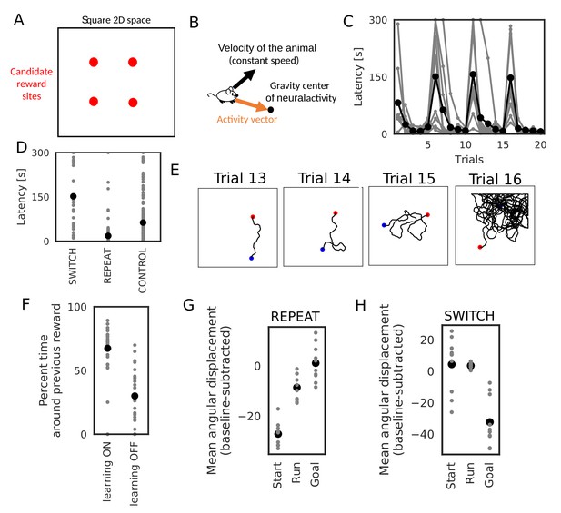
Learning goal-directed behavior in a 2-D space.
In all figures, gray color shows data from individual trials or simulation sets, and black color shows means over simulations. (A) The square two-dimensional space in the simulation. (B) Computational scheme for the animal’s motion. We modulated the fixed-length velocity vector with the activity vector from the animal’s current position to the center of mass of neural activity in the network. (C) Latency to reach the goal (N = 10 simulations sets). (D) Comparison of latency in SWITCH trials (trial 6, 11, 16), REPEAT trials (trial 2–5, 7–10, 12–15, 16–20), and control simulations in which we turned off learning (N = 160 trials for REPEAT, N = 30 trials for SWITCH, N = 200 trials for CONTROL). (E) Example trajectories of the animal. Blue and red circle shows start and goal positions, respectively. (F) Comparison of the percent time spent in the quadrant containing the previous reward site between SWITCH trials with and without learning (N = 30 trials for both). (G, H) Comparison of mean angular displacements between the activity vector and reference vectors at start, during run, and goal (N = 10 simulation sets). Reference vectors were directed to reward (start and run), or directed to the recent paths (goal). We subtracted the mean angular displacements calculated from control simulations in each behavioral state.
Tables
Correlations between parameters and biases to reverse direction.
Correlations (r) between the values of parameters (mean ISI and propagation speed of spike trains, parameters of short-term plasticity) and biases in recurrent synaptic weights toward the reverse direction are listed for Figures 3 and 4 together with the p-values.
| r | P | |
|---|---|---|
| 2 spikes, ISI – Mean bias | 0.386 | |
| 2 spikes, Speed – Mean bias | −0.252 | |
| 2 spikes, ISI – P(bias > 0) | −0.279 | |
| 2 spikes, Speed– P(bias > 0) | 0.156 | |
| 3 spikes, ISI – Mean bias | 0.315 | |
| 3 spikes, Speed – Mean bias | −0.503 | |
| 3 spikes, ISI – P(bias > 0) | −0.539 | |
| 3 spikes, Speed– P(bias > 0) | 0.108 | 0.00066 |
| 4 spikes, ISI – Mean bias | 0.125 | |
| 4 spikes, Speed – Mean bias | −0.616 | |
| 4 spikes, ISI – P(bias > 0) | −0.728 | |
| 4 spikes, Speed– P(bias > 0) | 0.104 | 0.00104 |
| 5 spikes, – Mean bias | 0.914 | |
| 5 spikes, – Mean bias | 0.236 | |
| 5 spikes, – Mean bias | −0.0455 | 0.151 |
| 5 spikes, – P(bias>0) | 0.869 | |
| 5 spikes, – P(bias>0) | 0.264 | |
| 5 spikes, – P(bias>0) | −0.0416 | 0.188 |
| 5 spikes, ISI – Mean bias | −0.0896 | 0.00459 |
| 5 spikes, Speed – Mean bias | −0.658 | |
| 5 spikes, ISI – P(bias > 0) | −0.817 | |
| 5 spikes, Speed– P(bias > 0) | 0.0280 | 0.376 |
Correlations between parameters and biases during run.
Correlations (r) between the values of parameters (mean peak firing rat and phase selectivity) and biases in recurrent synaptic weights toward the reverse direction are listed for Figure 5 and Figure 5—figure supplement 1 together with the p-values.
| Single-cell, Broad STDP | r | P |
|---|---|---|
| Peak firing rate – Mean bias | 0.958 | |
| Phase selectivity – Mean bias | −0.0506 | 0.11 |
| Peak firing rate – P(bias > 0) | 0.911 | |
| Phase selecitivity – P(bias > 0) | −0.0478 | 0.131 |
| 10 cells, Broad STDP | r | P |
| Peak firing rate – Mean bias | 0.979 | |
| Phase selectivity – Mean bias | −0.0337 | 0.287 |
| Peak firing rate – P(bias > 0) | 0.926 | |
| Phase selectivity – P(bias > 0) | −0.0241 | 0.447 |
| Single-cell, Narrow STDP | r | P |
| Peak firing rate – Mean bias | 0.909 | |
| Phase selectivity – Mean bias | 0.189 | |
| Peak firing rate – P(bias > 0) | 0.939 | |
| Phase selectivity – P(bias > 0) | 0.0982 | 0.00186 |
Additional files
-
Transparent reporting form
- https://doi.org/10.7554/eLife.34171.025


