Uncovering temporal structure in hippocampal output patterns
Figures
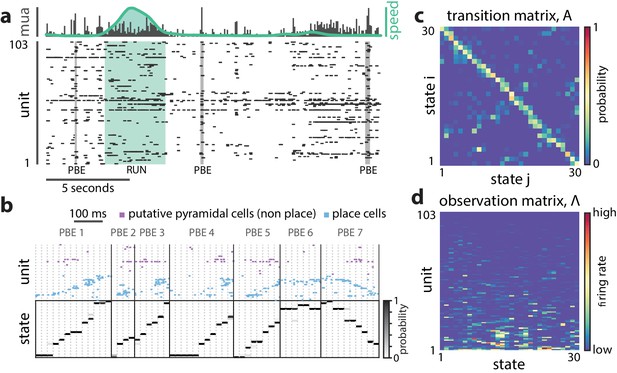
A hidden Markov model of ensemble activity during PBEs.
A hidden Markov model of ensemble activity during PBEs. (a) Examples of three PBEs and a run epoch. (b) Spikes during seven example PBEs (top) and their associated (30 state HMM-decoded) latent space distributions (bottom). The place cells are ordered by their place fields on the track, whereas the non-place cells are unordered. The latent states are ordered according to the peak densities of the lsPFs (lsPFs, see Materials and methods). (c) The transition matrix models the dynamics of the unobserved internally-generated state. The sparsity and banded-diagonal shape are suggestive of sequential dynamics. (d) The observation model of our HMM is a set of Poisson probability distributions (one for each neuron) for each hidden state. Looking across columns (states), the mean firing rate is typically elevated for only a few of the neurons and individual neurons have elevated firing rates for only a few states.
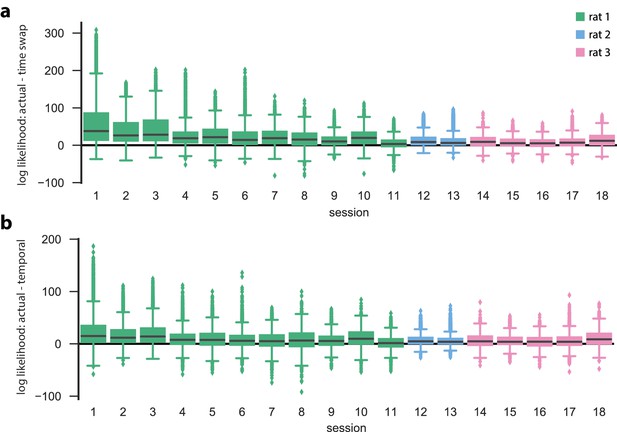
Hidden Markov models capture state dynamics beyond pairwise co-firing.
Actual cross-validated test data and surrogate test data evaluated in actual-data-optimized HMMs for all 18 linear track sessions. For each session, we performed five-fold cross validation to score the validation (=test) set in an HMM that was learned on the corresponding training set. In addition, two surrogate datasets of the validation data (obtained by either temporal shuffle or time-swap shuffle) were scored in the same HMM as the actual validation data. shuffles of each event and of each type were performed. (a) Difference between the data log likelihoods of actual and time-swap surrogate test events, evaluated in the actual train-data-optimized models. (b) Same as in (a), except that the differences between the actual data and the temporal surrogates are shown. For each of the sessions, the actual test data had a significantly higher likelihood than either of the shuffled counterparts (, Wilcoxon signed-rank test). Sessions are arranged first by animal, and then by number of PBEs, in decreasing order.
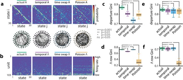
A hidden Markov model of ensemble activity during population burst events.
Models of PBE activity are sparse. We trained HMMs on neural activity during PBEs (in 20 ms bins), as well as on surrogate transformations of those PBEs. (a) (top) The transition matrices for the actual and surrogate PBE models with states ordered to maximize the transition probability from state to state . (bottom) Undirected connectivity graphs corresponding to the transition matrices. The nodes correspond to states (progressing clockwise, starting at the top). The weights of the edges are proportional to the transition probabilities between the nodes (states). The transition probabilities from state i to every other state except are shown in the interior of the graph, whereas for clarity, transition probabilities from state to itself, as well as to neighboring state are shown between the inner and outer rings of nodes (the nodes on the inner and outer rings represent the same states). (b) The observation matrices for actual and surrogate PBE models show the mean firing rate for neurons in each state. For visualization, neurons are ordered by their firing rates. (c) We quantified the sparsity of transitions from one state to all other states using the Gini coefficient of rows of the transition matrix for the example session in (a). Actual data yielded sparser transition matrices than shuffles. (d) The observation models—each neuron’s expected activity for each state—learned from actual data for the example session are significantly sparser than those learned after shuffling. This implies that as the hippocampus evolves through the learned latent space, each neuron is activeduring only a few states. (e) Summary of transition matrix sparsity and f. Observation model sparsity with corresponding shuffle data pooled over all sessions/animals. (***: , *: ; single session comparisons: realizations, Welch’s t-test; aggregated comparisons - sessions, Wilcoxon signed-rank test).
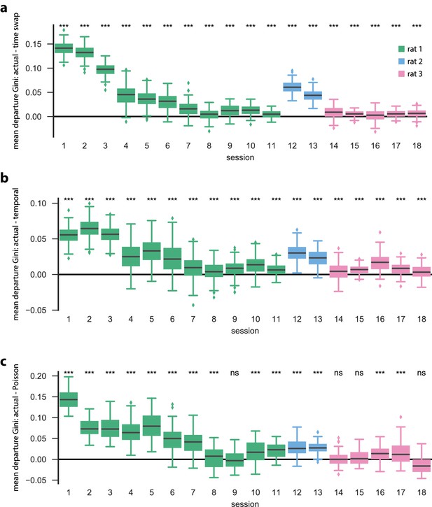
PBE model states typically only transition to a few other states.
We trained HMMs on neural activity during PBE (in 20 ms bins), and asked how sparse the resulting state transitions were. In particular, we calculated the Gini coefficient for each row of our state transition matrix, so that the Gini coefficient for a particular row reflects the sparsity of state transitions from that state (row) to all other states (so-called ‘departure sparsity’). A high (closeto one) Gini coefficient implies that the state is likely to only transition to a few other states, whereas a low (close to zero) Gini coefficient implies that the state is likely to transition to many other states. For each transition matrix, we computed the mean departure sparsity for initializations, and for shuffled counterparts for each of the surrogate datasets (a) time-swap shuffle, (b) temporal shuffle, (c) Poisson surrogate), and in each case we show the difference between the actual test data, and the surrogate test data. The actual data are significantly more sparse than both the temporal and time-swap surrogates for all sessions (, Mann–Whitney U test) and significantly more sparse than the Poisson surrogate for 14 of the 18 sessions (, Mann–Whitney U test).
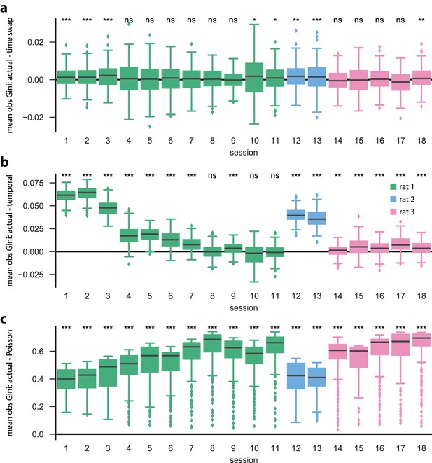
Each neuron is active in only a few model states.
Using the same PBE models and surrogate datasets ( shuffles each) as in Figure 2—figure supplement 2, we investigated the sparse participation of neurons/units in our models by calculating the Gini coefficient of each row (that is, for each unit) of the observation matrix. A high Gini coefficient implies that the unit is active in only a small number of states, whereas a low Gini coefficient implies that the unit is active in many states. For each initialization/shuffle, we calculate the mean Gini coefficient over all units, and the differences between those obtained using actual data and those obtained using surrogate data are shown: differences between actual and (a) time-swap, (b) temporal, and (c) Poisson surrogates. We find that the actual data are significantly more sparse than the temporal and Poisson surrogates for most of the sessions (p<0.001, Mann–Whitney U test), but that for many (10 out of 18) sessions, there is no significant difference between the mean row-wise observation sparsity of the actual data compared to the time-swap surrogate. This is an expected result, since the time-swap shuffle leaves the observation matrix largely unchanged.
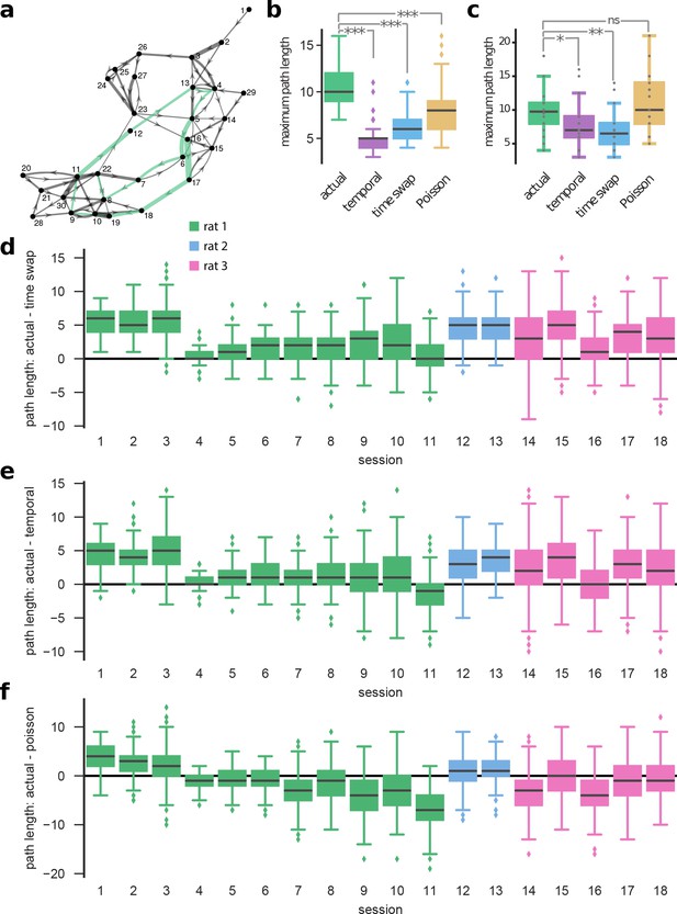
The sparse transitions integrate into long sequences through the state space.
We calculated the longest path within an unweighted directed graph corresponding to the transition matrices of HMMs, with nodes representing states and edges reflecting the transition probabilities (see Materials and methods). (a) The graph—displayed using the ‘force-directed layout’ (Fruchterman and Reingold, 1991)—represents a model trained on actual data. For illustration purposes, we ignored transition probabilities below 0.1. The green path shows the longest path in the example. (b) For this example session, we computed the maximum path length (the number of nodes in the longest path) for actual and corresponding shuffle datasets (temporal, time-swap, and Poisson) (initializations/shuffles). (c) The panel shows aggregate results built of median maximum path lengths from all sessions. We find that the actual data results in longer paths compared to time-swap (, Mann–Whitney U test) and temporal surrogate datasets (, Mann–Whitney U test). On the contrary, no significant difference is found in comparison with the Poisson datasets (, Mann–Whitney U test). Nevertheless, due to non-sparseness of the observation matrix for a Poisson model (Figure 2—figure supplement 3), in most instances these paths correspond to highly overlapping ensemble sequences. In panels (d–f), difference between maximum path lengths obtained from actual data and surrogate datasets are shown separately for all sessions: actual versus (d) time-swap, (e) temporal, and (f) Poisson. The data results in longer paths compared to time-swap and temporal shuffle datasets in most sessions (15 out of 18) (, Mann–Whitney U test), though in only five sessions compared to Poisson surrogate datasets.
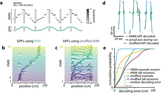
Latent states capture positional code.
Latent states capture positional code. (a) Using the model parameters estimated from PBEs, we decoded latent state probabilities from neural activity during periods when the animal was running. An example shows the trajectory of the decoded latent state probabilities during six runs across the track. (b) Mapping latent state probabilities to associated animal positions yields latent-state place fields (lsPFs) which describe the probability of each state for positions along the track. (c) Shuffling the position associations yields uninformative state mappings. (d) For an example session, position decoding during run periods through the latent space gives significantly better accuracy than decoding using the shuffled tuning curves. The dotted line shows the animal’s position during intervening non run periods. (e) The distribution of position decoding accuracy over all sessions () was significantly greater than chance. ().
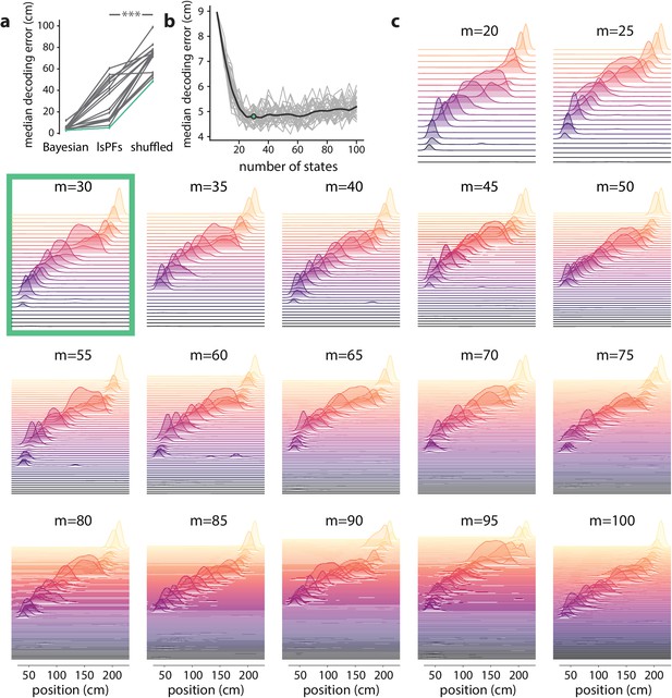
Latent states capture positional code over wide range of model parameters.
We investigated to what extent our PBE models encoded information related to the animal’s positional code by learning an additional mapping from the latent-state space to the animal’s position (resulting in a latent-space place field, lsPF), and then using this mapping, we decoded run epochs to position and assessed the decoding accuracy. (a) We computed the median position decoding accuracy (via the latent space) for each session on the linear track ( sessions) using cross validation. In particular, we learned a PBE model for each session, and then using cross validation we learned the latent space to animal position mapping on a training set, and recorded the position decoding accuracy on the corresponding test set by first decoding to the state space using the PBE model, and then mapping the state space to the animal position using the lsPF learned on the training set. The position decoding accuracy was significantly greater than chance for each of the 18 sessions (, Wilcoxon signed-rank test). (b) For an example session, we calculated the median decoding accuracy as we varied the number of states in our PBE model ( realizations per number of states considered). Gray curves show the individual realizations, and the black curve shows the mean decoding accuracy as a function of the number of states. The decoding accuracy is informative over a very wide range of number of states, and we chose states for the analysis in the main text. (c) For the same example session, we show the lsPF for different numbers of states. The lsPF are also informative over a wide range of number of states, suggesting that our analyses are largely insensitive to this particular parameter choice (the number of states). The coloration of the lsPF is only for aesthetic reasons.
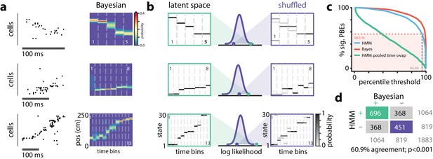
Replay Events Can Be Detected Via HMM Congruence.
(a) Example PBEs decoded to position using Bayesian decoding. (b) (left) Same examples decoded to the latent space using the learned HMM. (right) Examples decoded after shuffling the transition matrix, and (middle) the sequence likelihood using actual and shuffled models. (c) Effect of significance threshold on the fraction of events identified as replay using Bayesian decoding and model congruent events using the HMM approach. (d) Comparing Bayesian and model-congruence approaches for all PBEs recorded, we find statistically significant agreement in event identification (60.9% agreement, events from 18 sessions, , Fisher’s exact test two sided).
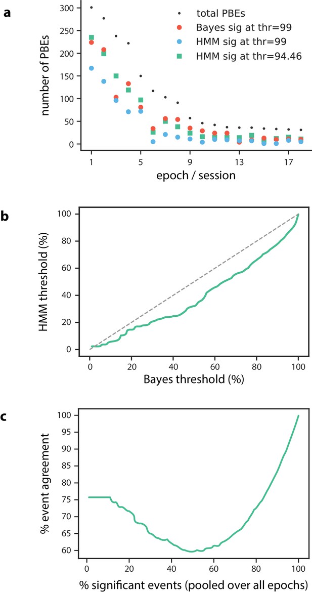
Number of significant PBEs.
(a) The number of Bayesian significant PBEs, as well as the total number of PBEs are shown for each session () when using a significance threshold of 99%. We find that 57% of PBEs (1064 of 1883) are Bayesian significant at this threshold. When using this same threshold for the model-congruence (HMM) significance testing, we find that only 35% of PBEs (651 of 1883) are model congruent. In order to compare the Bayesian and model-congruence approaches more directly, we therefore lowered the model-congruence threshold to 94.46%, at which point both methods had the same number of significant events (1064 of 1883). (b) For each Bayesian significance threshold, we can determine the corresponding model-congruence threshold that would result in the same number of significant PBEs. (c) Using the thresholds from (b) such that at each point, both Bayesian and model-congruence approaches have the same number of significant PBEs, we calculate the event agreement between the two approaches. We note that our chosen threshold of 57% significant events has among the worst agreement between the two approaches.
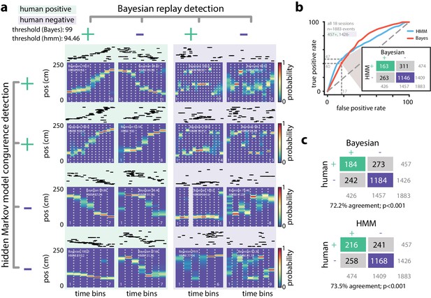
Comparing HMM congruence and Bayesian decoding in replay detection.
(a) Eight examples from one session show that Bayesian decoding and HMM model-congruence can differ in labeling of significant replay events. For each event, spike rasters (ordered by the location of each neuron’s place field) and the Bayesian decoded trajectory are shown. ‘+' (‘-') label corresponds to significant (insignificant) events. (left) Both methods can fail to label events that appear to be sequential as replay and (right) label events replay that appear non-sequential. (b) We recruited human scorers to visually inspect Bayesian decoded spike trains and identify putative sequential replay events. Using their identifications as labels, we can define an ROC curve for both Bayesian and HMM model-congruence which shows how detection performance changes as the significance threshold is varied. (inset) Human scorers identify 24% of PBEs as replay. Setting thresholds to match this value results in agreement of 70% between Bayesian and HMM model-congruence. (c) Using the same thresholds, we find % agreement between algorithmic and human replay identification. (All comparison matrices, , Fisher’s exact test two-tailed.).
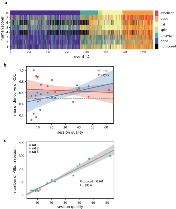
Human scoring of PBEs and session quality.
(a) Manual scoring results from eight human scorers (six individuals scored events, two individuals scored a subset of events). Events were presented to each participant in a randomized order, and individuals were allowed to go back to modify their results before submission. Here, events are ordered according to individual #8’s classifications. (b) The model-congruence (HMM) approach appearsto have higher accuracy when the session quality is higher (, ), which is consistent with our expectation that we need many congruent events in the training set in order to learn a consistent and meaningful model. (c) The session quality is strongly correlated with the number of PBEs recorded within a session (, ).
Modeling PBEs in open field.
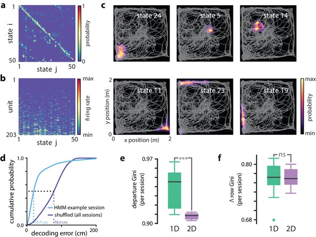
Modeling PBEs in open field. (a) The transition matrix estimated from activity detected during PBEs in an example session in the open field. (b) The corresponding observation model (203 neurons) shows sparsity similar to the linear track. (c) Example latent state place fields show spatially-limited elevated activity in two dimensions. (d) For an example session, position decoding through the latent space gives significantly better accuracy than decoding using the shuffled latent state place fields. (e) Comparing the sparsity of the transition matrices (mean Gini coefficient of the departure probabilities) between the linear track and open field reveals that, as expected, over the sessions we observed, the open field is significantly less sparse (), since the environment is less constrained. (f) In contrast, there is not a significant difference between the sparsity of the observation model (mean Gini coefficient of the rows) between the linear track and the open field. Note that the linear track models are sparser than in Figure 2 due to using 50 states rather than 30 to match the open field.
Open field PBE model states typically only transition to a few other states.
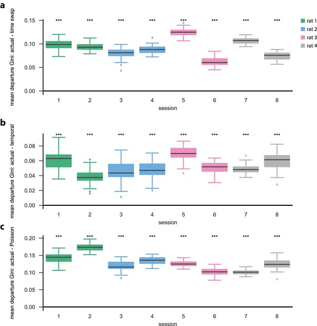
Similar to the linear track (one dimensional) case, we find that models learned on actual open field PBE data are significantly more sparse (here showing mean departure sparsity) than their shuffled ( shuffles) counterparts. This is true for each of the open field sessions (, Mann–Whitney U test). (a) Difference [in departure Gini coefficients] between actual and time-swap test data, (b) between actual and temporal test data, and c) between actual and Poisson surrogate data.
Each neuron is active in only a few model states in the open field.
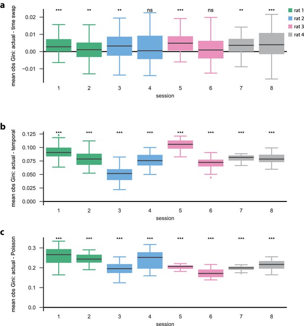
(a) Difference [in observation sparsity Gini coefficients across states] between actual and time-swap test data, (b) between actual and temporal test data, and (c) between actual and Poisson surrogate data. Similar to the linear track (one dimensional) case, we find that the observation sparsity across states for actual data are significantly greater than that of both the (b) temporal and (c) Poisson surrogates (for each session, , Mann–Whitney U test), and that (a) for some sessions, there are no significant differences between the actual and time-swap surrogates.
lsPF and position decoding in an open field.
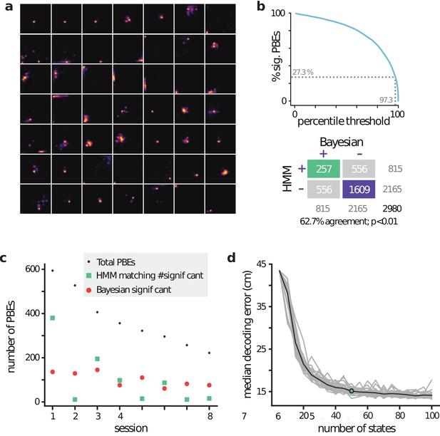
(a) lsPF for 49 of the 50 latent states from an example session. (b) (Top) Effect of model-congruence threshold on the number of significant PBEs. (Bottom) Comparison matrix between Bayesian replay detection and our model-congruence approach, where the threshold was chosen to match the total number of significant events pooled over all eight sessions. (c) Comparison between number of significant Bayesian events vs number of significant events using our model-congruence approach, when choosing the threshold as in (b). Sessions are ordered in decreasing numbers of total PBEs. Note that session one is a significant outlier, causing mismatches between many other sessions (2, 5, 7, 8), suggesting that matching on a per-session basis may be more appropriate in this case. (d) Median position decoding error (via the latent space and lsPF) was evaluated using cross-validation in an example session ( realizations for each model considered, shown in gray, mean shown in black), indicating that (i) the PBE-learned latent space encodes underlying spatial information, and (ii) that our PBE models are informative aboutthe underlying position over a wide range of numbers of states.
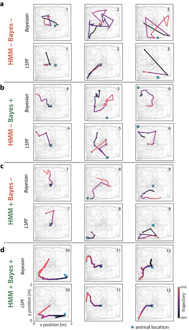
Examples of open field PBEs.
(a) Three example PBEs are shown that were classified as non-significant by both the Bayesian and model-congruence approaches. The top row shows the PBE decoded with place fields using a Bayesian decoder in 20 ms bins, with a 5 ms stride. The bottom row shows the same events, but decoded in 20 ms non-overlapping time bins using the lsPF. (b) Three example PBEs are shown that were classified as significant replay by the Bayesian approach, but not by the model-congruence approach. (c) Three example PBEs are shown that were classified as significant replay by the model-congruence approach, but not by the Bayesian approach. (d) Three example PBEs are shown that were classified as significant by both approaches.
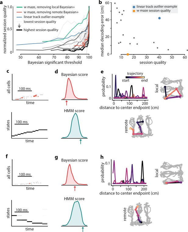
Extra-spatial structure.
Examples of remote replay events identified with HMM-congruence. We trained and evaluated HMMs on the events that were not Bayesian significant (residual events) to identify potential extra-spatial structure. (a) The normalized session quality drops as local-replay events above the Bayesian significance threshold are removed from the data. Each trace corresponds to one of the 18 linear track sessions, with the stroke width and the stroke intensity proportional to the baseline (all-events) session quality. The blue line identifies a session in which model quality drops more slowly, indicating the potential presence of extra-spatial information. The reduction in session quality for a W maze experiment with known extra-spatial information is even slower (green). When, instead, Bayesian-significant remote events are removed, rapid reduction in session quality is again revealed (red). (b) The lsPF-based median decoding errors are shown as a function of baseline session quality for all 18 linear track sessions. The blue dot indicates the outlier session from panel (a) with potential extra-spatial information: this session shows high decoding error combined with high session quality. Session quality of the W maze session is also indicated on the x-axis (decoding error is not directly comparable). (c–n) Two example HMM-congruent but not Bayesian-significant events from the W maze session are depicted to highlight the fact that congruence can correspond to remote replay. (c) Spikes during ripple with local place cells highlighted (top panel) and the corresponding latent state probabilities (bottom panel) decoded using the HMM show sequential structure (grayscale intensity corresponds to probability). (d) In this event, the Bayesian score relative to the shuffle distribution (top panel) indicates that the event is not-significant, whereas the HMM score relative to shuffles indicates (bottom panel) the ripple event is HMM-congruent. (e) Estimates of position using local place fields show jumpy, multi-modal a posteriori distributions over space in 1D (top left panel) and 2D (top right panel; distribution modes and time is denoted in color). Bayesian decoding using the remote environment place fields (bottom panel) indicates that the sample event is a remote replay. Note that in a typical experiment, only the local place fields would be available. (f–h) Same as (c–e), but for a different ripple event.
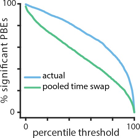
Temporal structure during a sleep period following object-location memory task.
Using cross validation, we calculate the HMM-congruence score (which ranges from 0 to 1) for test PBEs. For each event, we also calculate the score of a surrogate chosen using a pooled time-swap shuffle across all test events. The distribution of scores of actual events is significantly higher than that of the surrogate data (, Mann–Whitney U test).
Additional files
-
Transparent reporting form
- https://doi.org/10.7554/eLife.34467.021


