Learning place cells, grid cells and invariances with excitatory and inhibitory plasticity
- Technische Universität Berlin, Germany
Figures
Figure 1 with 2 supplements
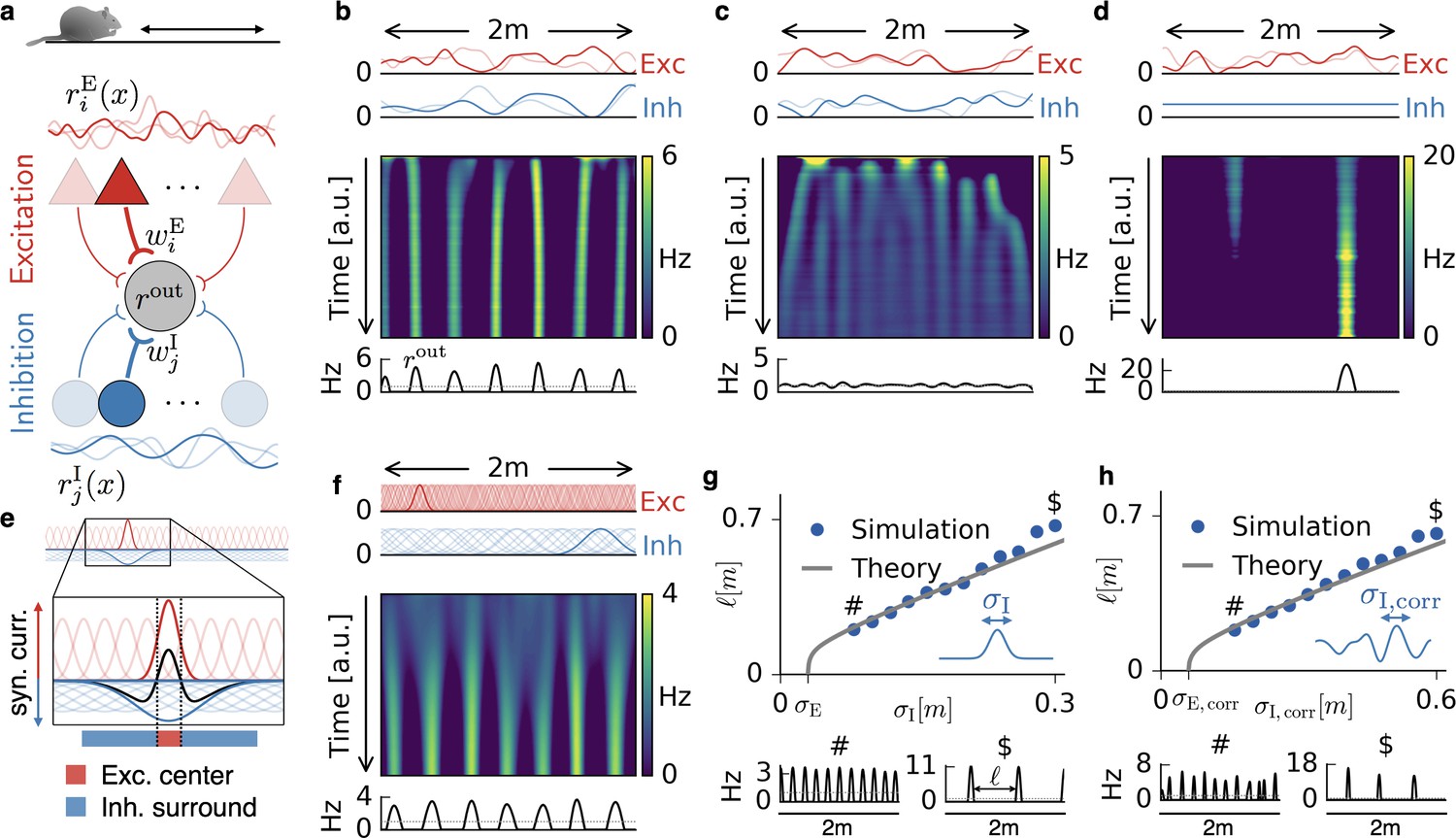
Emergence of periodic, invariant and single field firing patterns.
(a) Network model for a linear track. A threshold-linear output neuron (gray) receives input from excitatory (red) and inhibitory (blue) cells, which are spatially tuned (curves on top and bottom). (b) Spatially tuned input with smoother inhibition than excitation. The fluctuating curves (top) show two exemplary spatial tunings (one is highlighted) of excitatory and inhibitory input neurons. Interacting excitatory and inhibitory synaptic plasticity gradually changes an initially random response of the output neuron (firing rate ) into a periodic, grid cell-like activity pattern. (c) If the spatial tuning of inhibitory input neurons is less smooth than that of excitatory input neurons, the interacting excitatory and inhibitory plasticity leads to a spatially invariant firing pattern. The output neuron fires close to the target rate of 1 Hz everywhere. (d) For very smooth or spatially untuned inhibitory inputs, the output neuron develops a single firing field, reminiscent of a place cell. (e) The mechanism, illustrated for place cell-like input. When a single excitatory weight is increased relative to the others, the balancing inhibitory plasticity rule leads to an immediate increase of inhibition at the associated location. If inhibitory inputs are smoother than excitatory inputs, the resulting approximate balance creates a center surround field: a local overshoot of excitation (firing field) surrounded by an inhibitory corona. The next firing field emerges at a distance where the inhibition has faded out. Iterated, this results in a spatially periodic arrangement of firing fields. (f) Inputs with place field-like tuning. Gaussian curves (top) show the spatial tuning of excitatory and inhibitory input neurons (one neuron of each kind is highlighted, 20 percent of all inputs are displayed). A grid cell firing pattern emerges from an initially random weight configuration. (g) Grid spacing scales with inhibitory tuning width . Simulation results (dots) agree with a mathematical bifurcation analysis (solid). Output firing rate examples at the two indicated locations are shown at the bottom. (h) Inhibitory smoothness controls grid spacing; arrangement as in (d). Note that the time axes in (b,c,d,f) are different, because the speed at which the patterns emerge is determined by both the learning rates of the plasticity and the firing rate of the input neurons. We kept the learning rate constant and adjusted the simulation times to achieve convergence. Choosing identical simulation times, but different learning rates, leads to identical results (Figure 1—figure supplement 2). Rat clip art from [https://openclipart.org/detail/216359/klara; 2015].
Figure 1—figure supplement 1
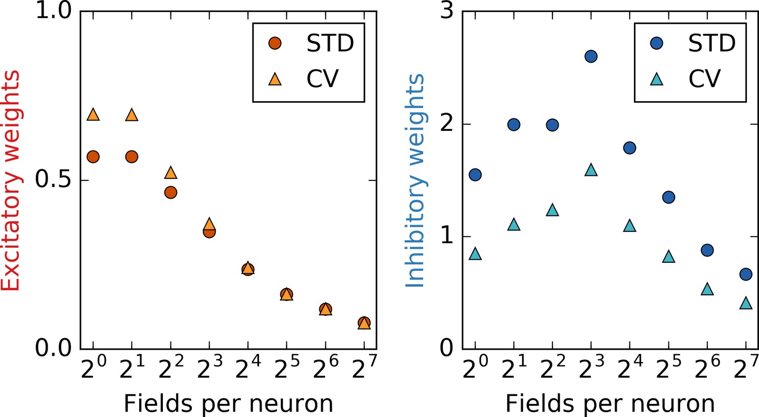
Statistics of the synaptic weights.
Depicted are the standard deviation (STD) and the coefficient of variation (CV) of excitatory (left) and inhibitory (right) weights as a function of the number of place fields per input neuron. The values are computed after the output neuron has established a stable grid pattern on a linear track. For excitatory weights, the CV decreases significantly with non-localized input. This indicates that different firing patterns in the output neuron are closer in ‘weight space’ for non-localized input. In other words, to obtain a different firing pattern, the weights must be modified by a lesser amount, that is, the configuration and thus the output pattern is less robust: An explanation for the defects in grids with non-localized input.
Figure 1—figure supplement 2
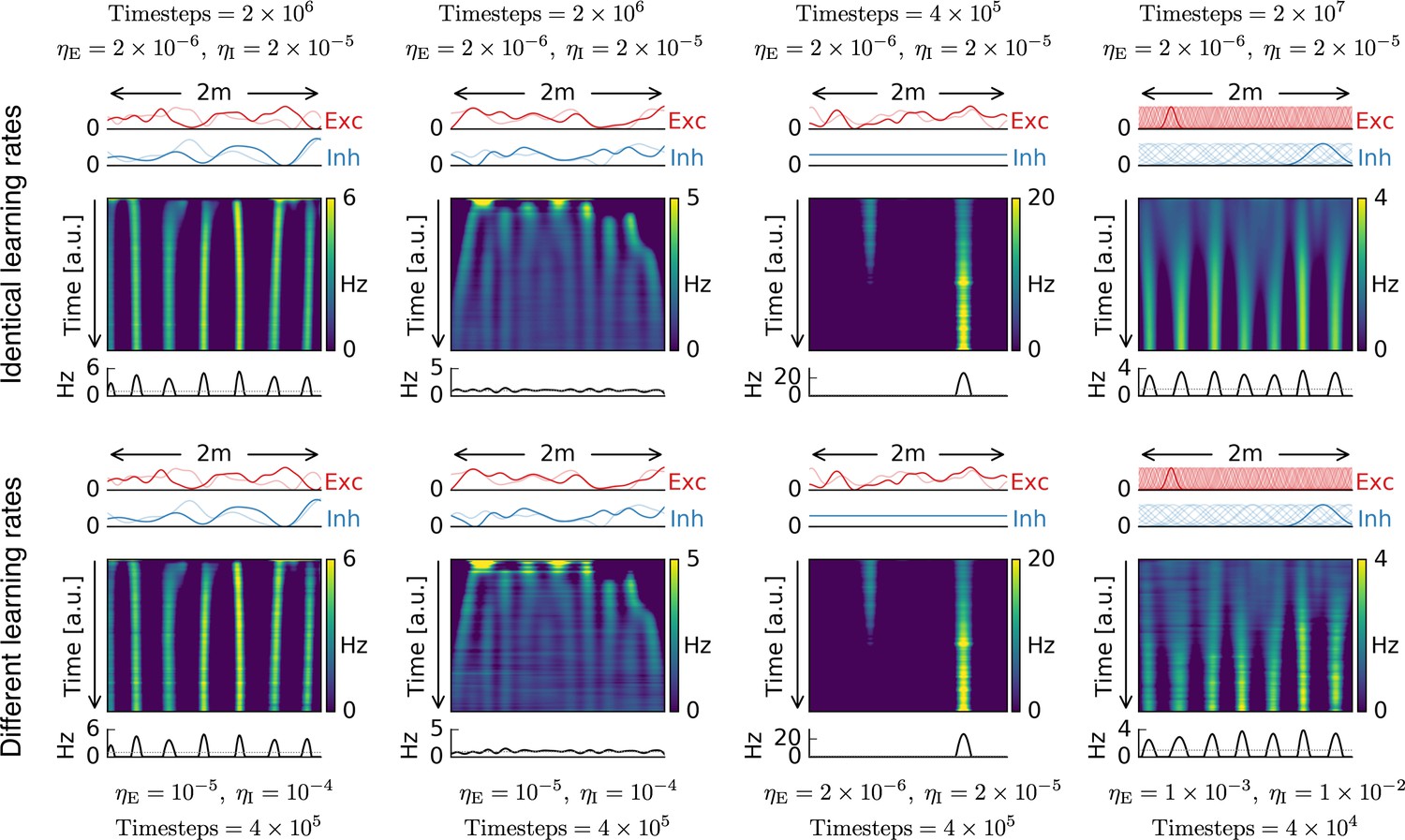
Different learning rates lead to identical results.
Top row: Each simulation with the same parameters as in Figure 1. Number of time steps and learning rates are indicated close to each plot.Bottom row: Same simulations as in top row, but with different excitatory and inhibitory learning rates and different number of simulation time steps.The two rows show basically identical time evolutions for the firing pattern of the output cell.As expected from the mathematical analysis, scaling the excitatory and inhibitory learning rates does not have an influence on the firing pattern of the output neuron, as long as learning is sufficiently slow.
Figure 2 with 6 supplements
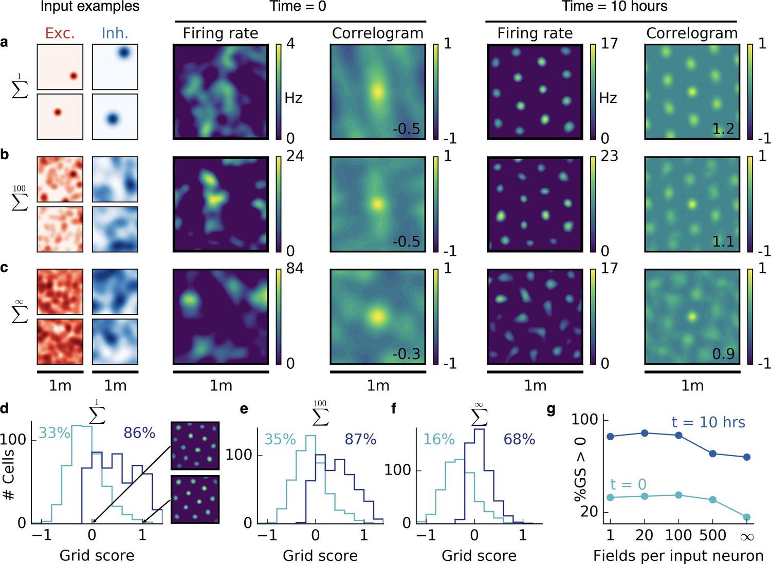
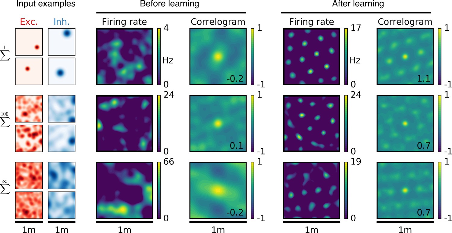
Emergence of two-dimensional grid cells.
(a,b,c) Columns from left to right: Spatial tuning of excitatory and inhibitory input neurons (two examples each); spatial firing rate map of the output neuron and corresponding autocorrelogram before and after spatial exploration of 10 hr. The number on the correlogram shows the associated grid score. Different rows correspond to different spatial tuning characteristics of the excitatory and inhibitory inputs. For all figures the spatial tuning of inhibitory input neurons is smoother than that of excitatory input neurons. (a) Each input neuron is a place cell with random location. (b) The tuning of each input neuron is given as the sum of 100 randomly located place fields. (c) The tuning of each input neuron is a random smooth function of the location. This corresponds to the sum of infinitely many randomly located place fields. Before learning, the spatial tuning of the output neuron shows no symmetry. After 10 hr of spatial exploration the output neuron developed a hexagonal pattern. (d) Grid score histogram for 500 output cells with place cell-like input. Before learning (light blue), 33% of the output cells have a positive grid score. After 10 hr of spatial exploration (dark blue), this value increases to 86%. Two example rate maps are shown. The arrows point to the grid score of the associated rate map. Even for low grid scores the learned firing pattern looks grid-like. (e,f) Grid score histograms for input tuning as in (b,c), arranged as in (d). (g) Fraction of neurons with positive grid score before (light blue) and after learning (dark blue) as a function of the number of fields per input neuron. Note that to learn within 10 hr of exploration time, we used different learning rates for different input scenarios. Using identical learning rates for all input scenarios but adjusting the simulation times to achieve convergence leads to identical results (Figure 2—figure supplement 6).
Figure 2—figure supplement 1
Influence of random simulation parameters on the final grid pattern.
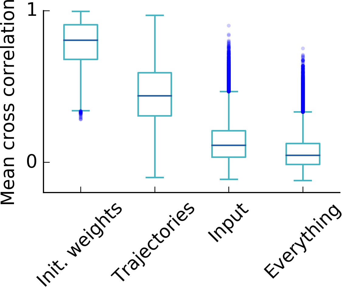
Box plot of the cross correlations of the rate maps after learning of 500 simulations (i.e. cross correlations). For each set of 500 simulations, only the parameter that is indicated on the axis was varied. A high cross correlation indicates that different simulations lead to similar grids and thus points towards a low influence of the varied parameter on the final grid pattern. We conclude that the influence on the final grid pattern in decreasing order is given by the parameters: Initial synaptic weights, trajectory of the rat, input tuning (i.e. locations of the randomly located input tuning curves). As expected, the correlation is lowest, if all parameters are different in each simulation (rightmost box). Each box extends from the first to the third quartile, with a dark blue line at the median. The lower whisker reaches from the lowest data point still within 1.5 IQR of the lower quartile, and the upper whisker reaches to the highest data point still within 1.5 IQR of the upper quartile, where IQR is the inter quartile range between the third and first quartile. Dots show flier points. See Appendix 1 for details on how trajectories, synaptic weights and inputs are varied.
Figure 2—figure supplement 2

Using different input statistics for different populations also leads to hexagonal firing patterns.
(a) Arrangement as in Figure 2a but with place cell-like excitatory input and sparse non-localized inhibitory input (sum of 50 randomly located place fields). A hexagonal pattern emerges, comparable with that given in Figure 2a,b,c. (b) Grid score histogram of 500 realizations with mixed input statistics as in (a). Arrangement as in Figure 2d.
Figure 2—figure supplement 3
Boundary effects in simulations with place field-like input.
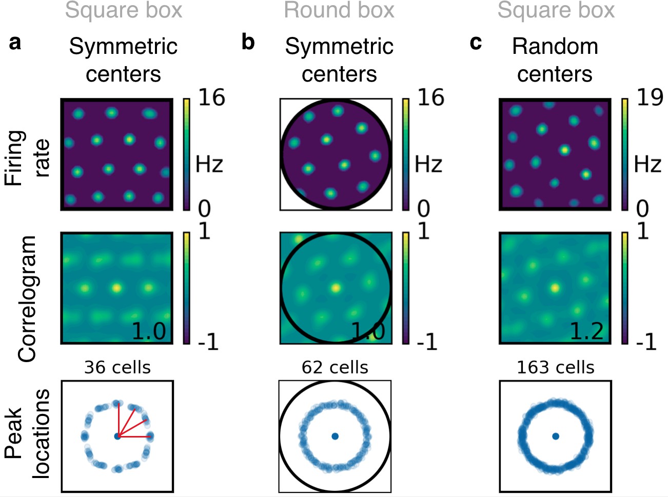
(a) Simulations in a square box with input place fields that are arranged on a symmetric grid. From top to bottom: Firing rate map and corresponding autocorrelogram for an example grid cell; peak locations of 36 grid cells. The clusters at orientation of 0, 30, 60 and 90 degrees (red lines) indicate that the grids tend to be aligned to the boundaries. (b) Simulations in a circular box with input place fields that are arranged on a symmetric grid. Arrangement as in (a). The grids show no orientation preference, indicating that the orientation preference in (a) is induced by the square shape of the box. (c) Simulations in a square box with input place fields that are arranged on a distorted grid (see Figure 2—figure supplement 5). Arrangement as in (a). The grids show no orientation preference, indicating that the influence of the boundary on the grid orientation is small compared with the effect of randomness in the location of the input centers.
Figure 2—figure supplement 4
Weight normalization is not crucial for the emergence of grid cells.
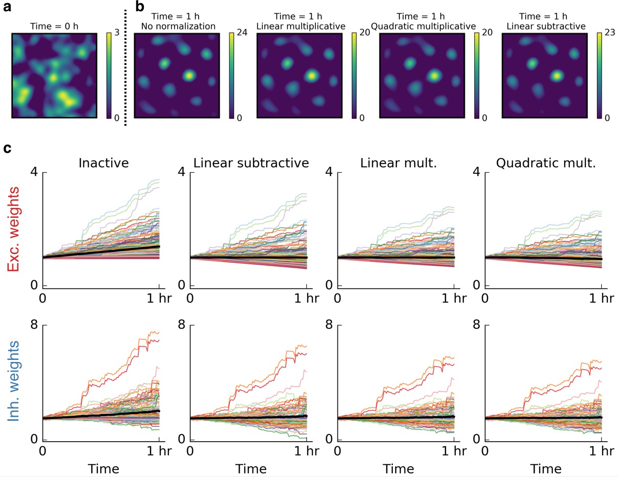
In all simulations in the main text we used quadratic multiplicative normalization for the excitatory synaptic weights – a conventional normalization scheme. This choice was not crucial for the emergence of patterns. (a) Firing rate map of a cell before it started exploring its surroundings. (b) From left to right: Firing rate of the output cell after 1 hr of spatial exploration for inactive, linear multiplicative, quadratic multiplicative and linear subtractive normalization. (c) Time evolution of excitatory and inhibitory weights for the simulations shown in (b). The colored lines show 200 individual weights. The black line shows the mean of all synaptic weights. From left to right: Inactive, linear multiplicative, quadratic multiplicative and linear subtractive normalization. Without normalization, the mean of the synaptic weights grows strongest and would grow indefinitely. On the normalization schemes: Linear multiplicative normalization keeps the sum of all weights constant by multiplying each weight with a factor in each time step. Linear subtractive normalization keeps the sum of all weights roughly constant by adding or subtracting a factor from all weights and ensuring that negative weights are set to zero. Quadratic multiplicative normalization is explained in Materials and methods.
Figure 2—figure supplement 5
Distribution of input fields.
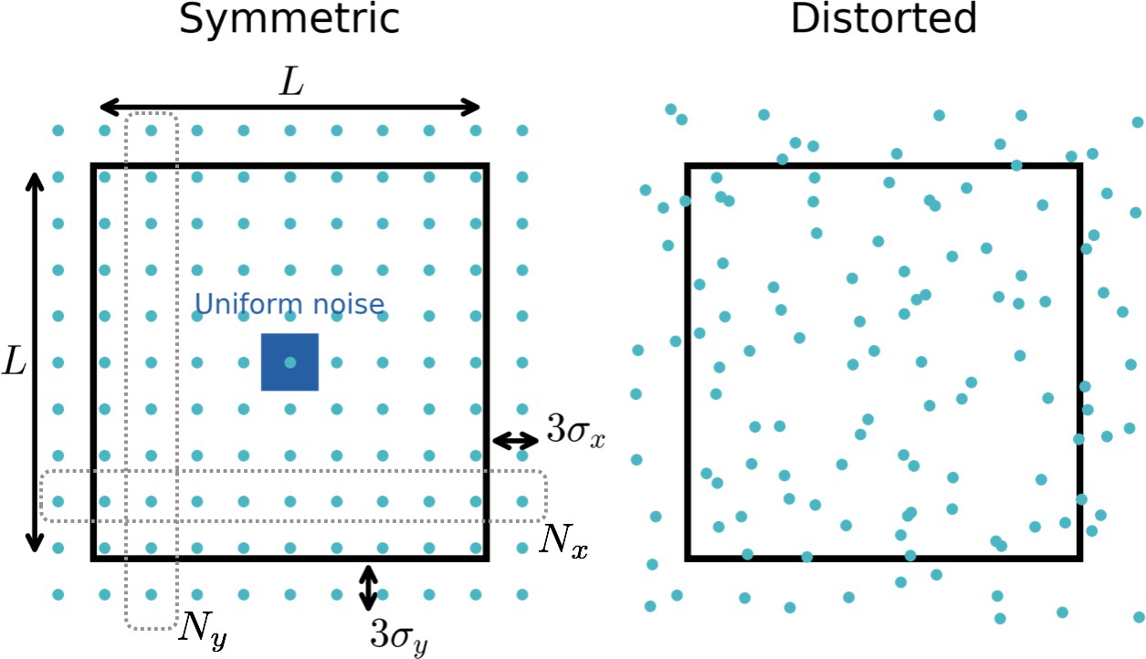
Black square box: Arena in which the simulated rat can move (side length ). Blue circles: Locations of input firing fields. To create random place field locations that cover the space densely, we use locations from a distorted lattice. To this end we first create a symmetric lattice with locations along the -direction and locations along the -direction. To reduce boundary effects, these centers can lie a certain distance outside the boundary (typically taken as threefold the width of the Gaussian input fields). We then add noise from a uniform distribution (blue square) to each location and obtain a distorted lattice (right). See Appendix 1 for more details on the choice of input functions.
Figure 2—figure supplement 6
Different learning rates lead to identical results.
This is the same figure as Figure 2a,b,c but with identical learning rates for all three input scenarios: , . To obtain similar results to those in Figure 2, we need to increase the simulation times. The exploration times for the three scenarios, from top to bottom, are: 335, 10 and 50 hr. Longer simulation times are needed for inputs with lower mean firing rate, because this corresponds to an effectively lower learning rate; compare to mathematical analysis. Note that 100 fields per neurons have a larger mean firing rate than the Gaussian random fields, because the Gaussian random fields are scaled to have a mean firing rate of 0.5 Hz (see Materials and methods). As in in one dimension, scaling the excitatory and inhibitory learning rates does not have an influence on the firing pattern of the output neuron, as long as learning is sufficiently slow. Note that the patterns here are not identical to the patterns in Figure 2 because of a different random initialization.
Figure 3 with 3 supplements
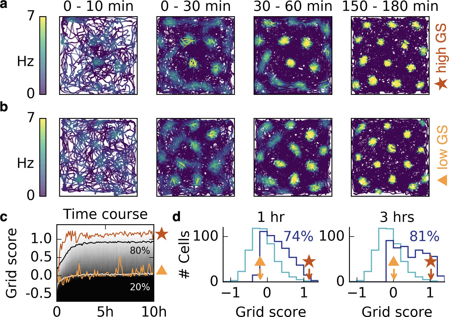
Grid patterns form rapidly during exploration and remain stable for many hours.
(a,b) Rat trajectories with color-coded firing rate of a cell that receives place cell-like input. The color depicts the firing rate at the time of the location visit, not after learning. Bright colors indicate higher firing rates. The time interval of the trajectory is shown above each plot. Initially all synaptic weights are set to random values. Parts (a) and (b) show two different realizations with a good (red star) and a bad (orange triangle) grid score development. After a few minutes a periodic structure becomes visible and enhances over time. (c) Time course of the grid score in the simulations shown in (a) (red) and (b) (orange). While the periodic patterns emerge within minutes, the manifestation of the final hexagonal pattern typically takes a couple of hours. Once the pattern is established it remains stable for many hours. The gray scale shows the cumulative histogram of the grid scores of 500 realizations (black = 0, white = 1). The solid white and black lines indicate the 20% and 80% percentiles, respectively. (d) Histogram of grid scores of the 500 simulations shown in (c). Initial histogram in light blue, histogram after 1 hr and after 3 hr in dark blue. Numbers show the fraction of cells with positive grid score at the given time. Rat trajectories taken from Sargolini et al., 2006b).
Figure 3—figure supplement 1
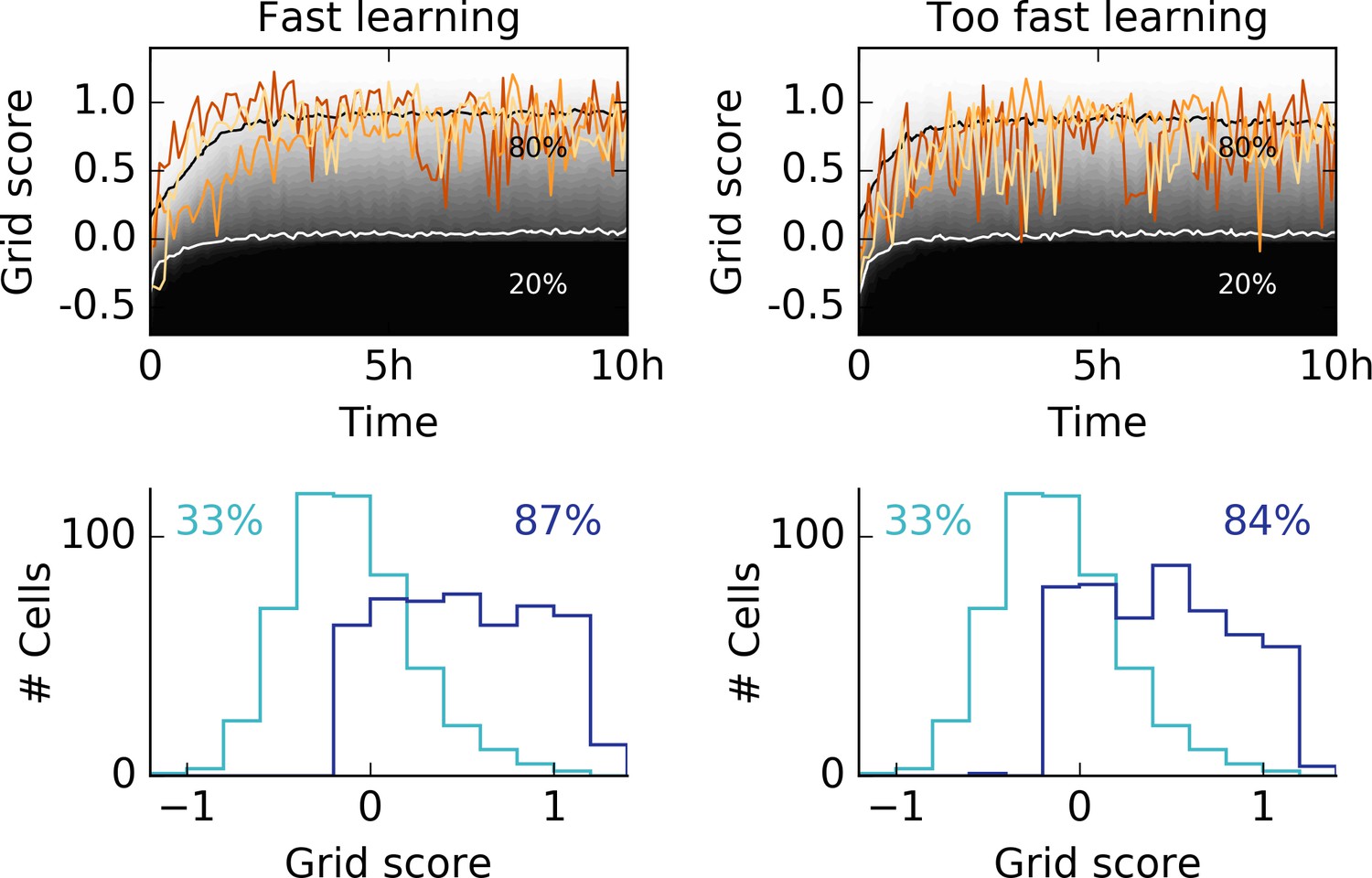
Learning too fast leads to unstable grids.
We showed that stable grid patterns emerge within minutes of behavioral rat trajectories (Figure 3) for high learning rates. Our model requires thorough spatial exploration of the rat, before significant weight changes occur. Accordingly, no stable patterns should emerge if the learning rate of the rat is too high. Left column: Same data as shown in Figure 3c with three different individual traces (top). Grid score histogram of 500 realizations before (light blue) and after 10 hr of spatial exploration (dark blue). Right column: The same simulations as shown on the left, but with twice the learning rates for excitatory and inhibitory synapses. The high learning rate leads to flickering unstable grids, as expressed in the large fluctuations in the grid score. The histogram after 10 hr of spatial exploration shows that fewer cells develop a hexagonal pattern if the learning rates are very high.
Figure 3—figure supplement 2

Influence of input remapping on grid patterns.
(a) A grid is learned from random initial weights and place cell-like input. After 1 hr the grid pattern is apparent. After 5 hr we remap a fraction (number above arrows) of the input, that is, the field locations of a fraction of place fields are changed to new random locations. A remapping fraction of 0 indicates that the input is unchanged and 1 indicates that all input neurons have a new place field location. The synaptic weights are not changed in this ‘input remapping’. After the remapping, the rat explores and continues learning. For all four remapping scenarios, a periodic pattern is visible shortly after the remapping. For remapping fractions less than 1, it occurs faster than during the initial learning from random weights. (b) Time courses of the grid scores for four different input remapping fractions as in (a) (Remap. frac.; shown above). The gray scale shows the cumulative histogram of the grid scores of 500 realizations (black = 0, white = 1). The solid white and black lines indicate the 20% and 80% percentiles, respectively. Colored lines show three individual traces. The red traces correspond to the simulations shown in (a). Varying a substantial fraction of the input often does not destroy the hexagonality of the grid patterns: Note the small dip in the 80% percentile for a remapping fraction of 0.5. (c) Time course of the Pearson correlation of a developing rate map with the rate map of the same simulation at 5 hr (right before the input was modified) for the same simulations as in (b), using the same color scheme and labeling. The stronger the input remapping, the lower the correlation of the grid after remapping with the grid before remapping. Note that the grid spacing is comparable for all grids, because the spatial autocorrelation length of the input is not modified during the remapping. Thus, for complete input remapping (fraction = 1) the new grid could be realigned with the old grid by a rotation and a phase shift.
Figure 3—figure supplement 3
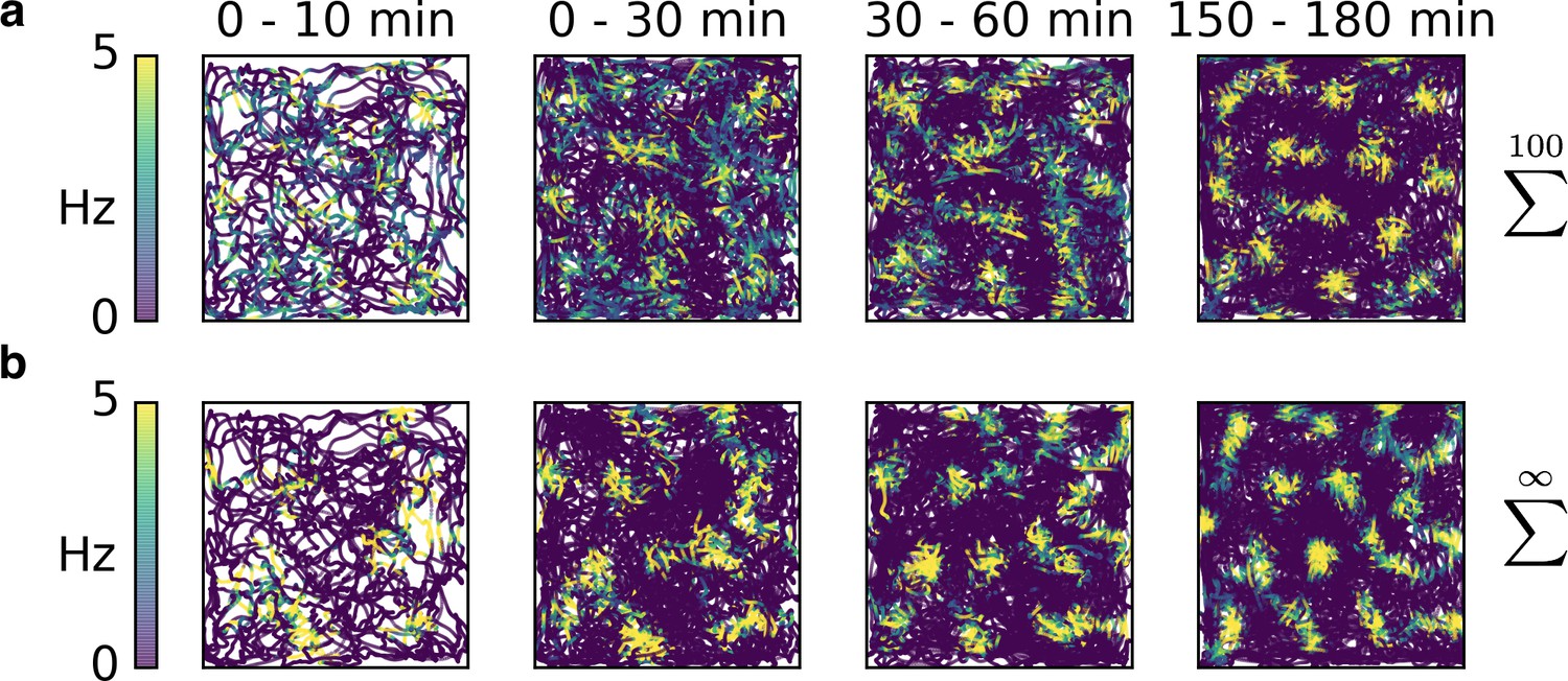
Rapid development of grid patterns from non-localized input.
(a) Sparse non-localized input (sum of 100 randomly located place fields) as in Figure 2b. (b) Dense non-localized input (random function with fixed spatial smoothness) as in Figure 2c. While the emergence of the final patterns takes roughly an hour – and thus longer than for place cell-like inputs (Figure 3) – the early firing fields are still present in the final grid, as observed in experiments (Hafting et al., 2005).
Figure 4
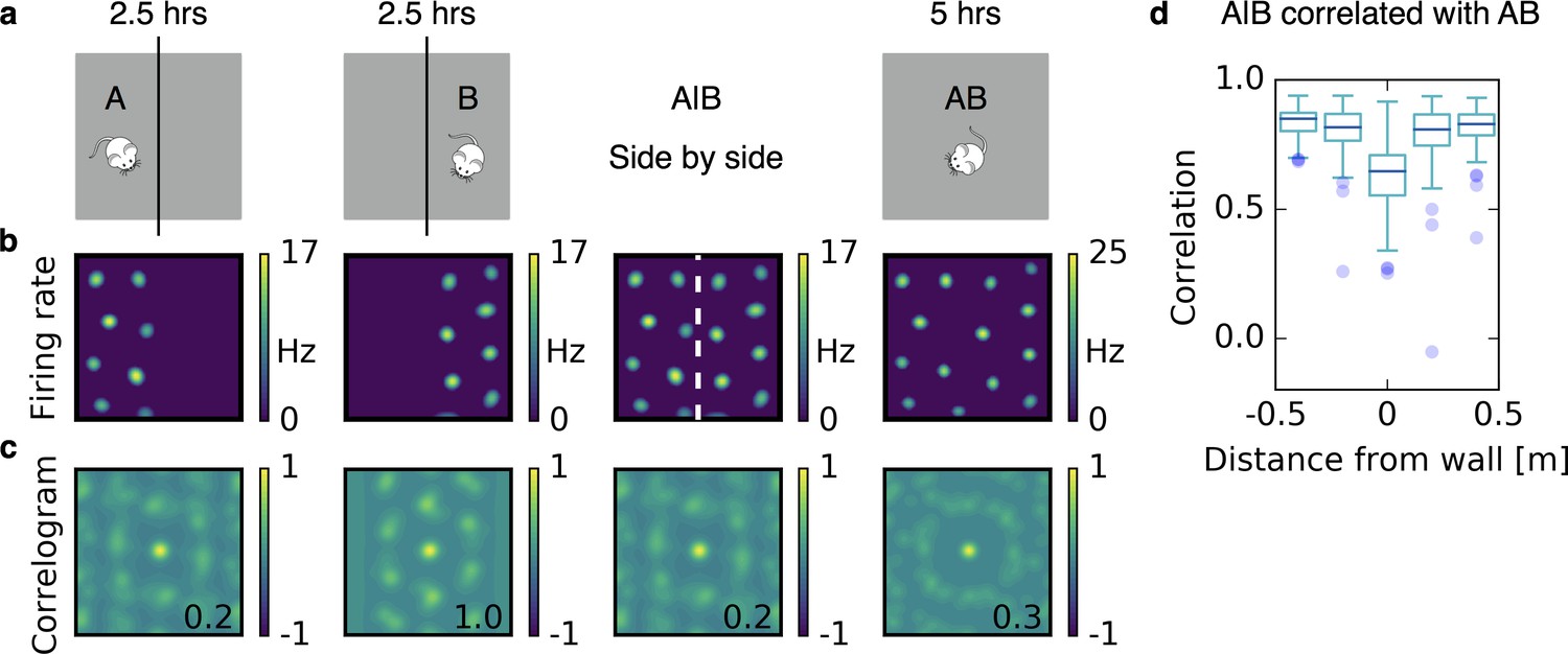
Grids coalesce in contiguous environments.
(a) Illustration of the experiment. A quadratic arena (gray box) is divided into two rectangular compartments by a wall (black line). The animal explores one compartment (A) and then the other compartment (B) for 2.5 hr each. Then the wall is removed and the rat explores the entire arena (AB) for 5 hr. (b) Firing rate maps. From left to right: After learning in A; after learning in B; the maps from A and B shown side by side (A|B); after learning in AB. (c) Autocorrelograms of the rate maps shown in (b). The number inside the correlogram shows the grid score. (d) Box plot of the correlations of the firing rate map A|B with the firing rate map AB as a function of distance from the partition wall. Close to the partition wall the correlation is low, far away from the partition wall it is high. This indicates that grid fields rearrange only locally. Each box extends from the first to the third quartile, with a dark blue line at the median. The lower whisker reaches from the lowest data point still within 1.5 IQR of the lower quartile, and the upper whisker reaches to the highest data point still within 1.5 IQR of the upper quartile, where IQR is the inter quartile range between the third and first quartile. Dots show flier points. Data: 100 realizations of experiments as in (a,b,c). For simulation details see Appendix 1. Mouse clip art from lemmling, https://openclipart.org/detail/17622/simple-cartoon-mouse-1; 2006.
Figure 5 with 1 supplement
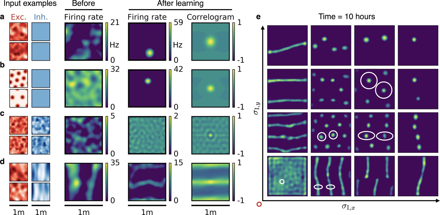
Emergence of spatially tuned cells of diverse symmetries.
(a,b,c,d) Arrangement as in Figure 2. (a,b) Place cells emerge if the inhibitory autocorrelation length exceeds the box length or if the inhibitory neurons are spatially untuned. The type of tuning of the excitatory input is not crucial: Place cells develop for non-localized input (a) as well as for grid cell input (b). (c) The output neuron develops an invariance if the spatial tuning of inhibitory input neurons is less smooth than the tuning of excitatory input neurons. (d) Band cells emerge if the spatial tuning of inhibitory input is asymmetric, such that its autocorrelation length is larger than that of excitatory input along one direction (here the -direction) and smaller along the other (here the -direction). (e) Overview of how the shape of the inhibitory input tuning determines the firing pattern of the output neuron. Each element depicts the firing rate map of the output neuron after 10 hr. White ellipses of width and in and direction indicate the direction-dependent standard deviation of the spatial tuning of the inhibitory input neurons. For simplicity, the width of the excitatory tuning fields, , is the same in all simulations. It determines the size of the circular firing fields. The red circle at the axis origin is of diameter .
Figure 5—figure supplement 1

Arrangement of firing fields for asymmetric input.
(a) For ellipsoidal spatial autocorrelation structures of inhibitory input (blue line), we observed band cell-like firing patterns or stretched grids (Figure 5e). Interestingly, the resulting patterns alternate between two different symmetries. This can be understood by two competing arrangements of ellipsoids. (b) A dense packing of ellipsoids maximizes the area with non-zero firing and is favored by the inhibitory learning rule. This leads to stretched grids. (c) Maximizing the overlap between excitatory input fields is favored by the excitatory learning rule and leads to quadratic grids with different periodicities along different directions. (d) Some simulations show a combination of both patterns; compare Figure 5e. The observed alignment of excitatory firing fields in (c) is particularly favored, if inhibition is very smooth along one direction. This could lead to alignment of the head direction of individual grid fields in the simulations shown in Figure 6.
Figure 6 with 2 supplements
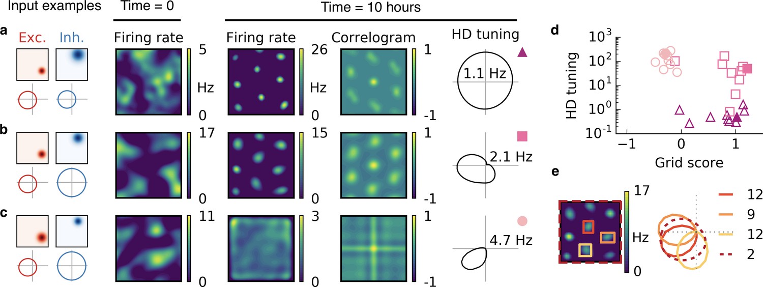
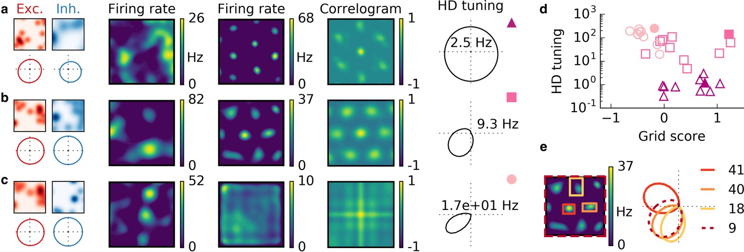
Combined spatial and head direction tuning.
(a,b,c) Columns from left to right: Spatial tuning and head direction tuning (polar plot) of excitatory and inhibitory input neurons (one example each); spatial firing rate map of the output neuron before learning and after spatial exploration of 10 hr with corresponding autocorrelogram; head direction tuning of the output neuron after learning. The numbers in the polar plots indicate the peak firing rate at the preferred head direction after averaging over space. (a) Wider spatial tuning of inhibitory input neurons than of excitatory input neurons combined with narrower head direction tuning of inhibitory input neurons leads to a grid cell-like firing pattern in space with invariance to head direction, that is, the output neuron fires like a pure grid cell. (b) The same spatial input characteristics combined with head direction-invariant inhibitory input neurons leads to grid cell-like activity in space and a preferred head direction, that is, the output neuron fires like a conjunctive cell. (c) If the spatial tuning of inhibitory input neurons is less smooth than that of excitatory neurons and the concurrent head direction tuning is wider for inhibitory than for excitatory neurons, the output neuron is not tuned to space but to a single head direction, that is, the output neuron fires like a pure head direction cell. (d) Head direction tuning and grid score of 10 simulations of the three cell types. Each symbol represents one realization with random input tuning. The markers correspond to the tuning properties of the input neurons as depicted in (a,b,c): grid cell (triangles), conjunctive cell (squares), head direction cell (circles). The values that correspond to the output cells in (a,b,c) are shown as filled symbols. (e) In our model, the head direction tuning of individual grid fields is sharper than the overall head direction tuning of the conjunctive cell. Depicted is a rate map of a conjunctive cell (left) and the corresponding head direction tuning (right, dashed). For three individual grid fields, indicated with colored squares, the head direction tuning is shown in the same polar plot. The overall tuning of the grid cell (dashed) is a superposition of the tuning of all grid fields. Numbers indicate the peak firing rate (in Hz) averaged individually within each of the four rectangles in the rate map.
Figure 6—figure supplement 1
Cells with combined spatial and head direction tuning with input tuning that is given by the sum of 20 randomly located Gaussian ellipsoids.
Arrangement as in Figure 6.
Figure 6—figure supplement 2
Head direction tuning of individual grid fields is difficult to assess from grid cells with few firing fields.
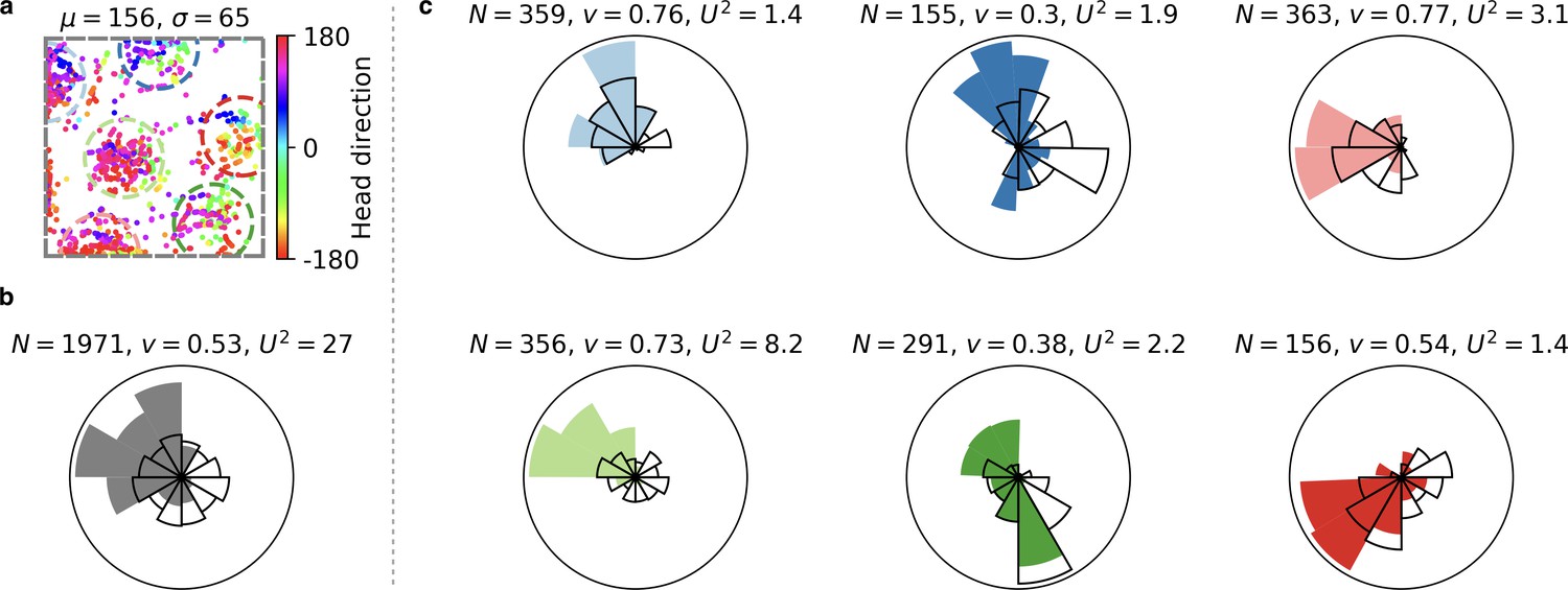
(a) Spike locations of a grid cell color-coded with the head direction of the rat at the moment the respective spike was fired. Circular mean and circular standard deviation of head directions at spike firing (‘spike head directions’ in the following) shown above. (b) Polar histogram of spike head directions (filled fan) and trajectory head directions (black fan) for all spikes of the grid cell. : Number of spikes. : Sum of unit vectors whose orientation is given by the spike head directions, normalized by . The larger this number, the more precise the head direction tuning. : Watson’s value (Appendix 1). The larger this number, the more the distribution of spike head directions deviates from the distribution of trajectory head directions. (c) Same arrangement as in (b) but for individual grid fields. Each plot corresponds to a different grid field. The colors of the filled fans correspond to the colors of the circles around grid fields in (a). Only spikes within these circles are considered. Individual grid fields often exhibit a sharper head direction tuning than the entire cell; compare the larger values. However, the trajectory often exhibits a strong head direction bias; compare the directionality of black fans. The head direction tuning of a grid field tends to align with this bias; compare the smaller values. Quantitative statements about the head direction tuning of individual grid fields would be easier for cells with more firing fields, because the head direction bias of rodents is less pronounced in central parts of the arena (Rubin et al., 2014); compare the grid field in the light green circle. From the publicly available data, we did not come to a conclusive answer on the tuning of individual grid fields. Data obtained from (Sargolini et al., 2006a; Sargolini et al., 2006b).
Figure 7
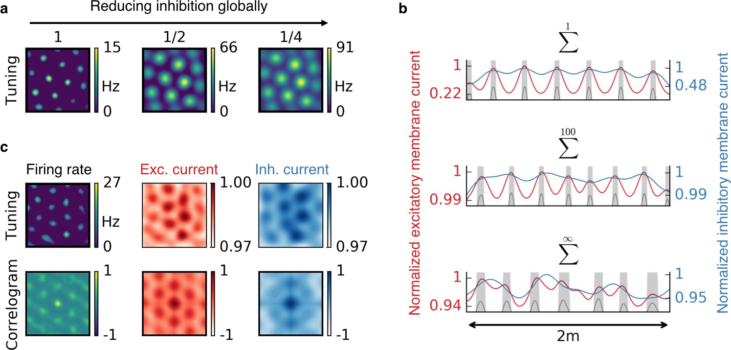
Effect of reduced inhibition on grid cell properties.
(a) Reducing the strength of inhibitory synapses to a fraction of its initial value (from left to right: 1, 1/2, 1/4) leads to larger grid fields but unchanged grid spacing in our model. In continuous attractor network models, the same reduction of inhibition would affect not only the field size but also the grid spacing. (b) Excitatory (red) and inhibitory (blue) membrane current to a cell with grid-like firing pattern (gray) on a linear track. The currents are normalized to a maximum value of 1. Different rows correspond to different spatial tuning characteristics of the input neurons. From top to bottom: Place cell-like tuning, sparse non-localized tuning (sum of 100 randomly located place fields), dense non-localized tuning (Gaussian random fields). Peaks in excitatory membrane current are co-localized with grid fields (shaded area) for all input statistics. In contrast, the inhibitory membrane current is not necessarily correlated with the grid fields for non-localized input. Moreover, the dynamic range of the membrane currents is reduced for non-localized input. A reduction of inhibition as shown in (a) corresponds to a lowering of the inhibitory membrane current. (c) Excitatory and inhibitory membrane current to a grid cell receiving sparse non-localized input (sum of 100 randomly located place fields) in two dimensions. Top: Tuning of output firing rate, normalized excitatory and inhibitory membrane current. Bottom: Autocorrelograms thereof. The grid pattern is more apparent in the spatial tuning of the excitatory membrane current than in the inhibitory membrane current.
Figure 8
Results of the mathematical analysis.
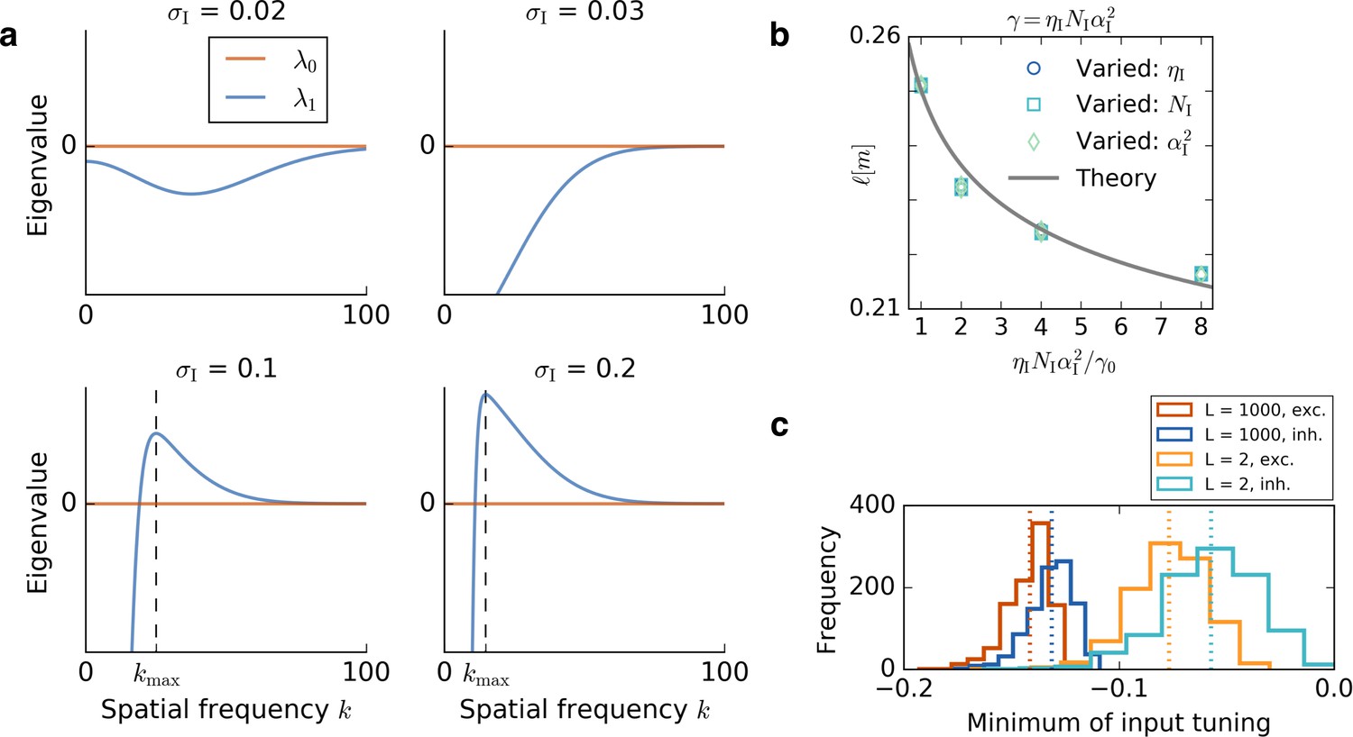
(a) The eigenvalue spectrum for the eigenvalues of Equation 72 for an excitatory tuning of width . The first eigenvalue is always 0. If the inhibitory tuning is more narrow than the excitatory tuning, that is, , the second eigenvalue is negative for every wavevector . For the eigenvalue spectrum has a unique positive maximum , that is, a most unstable spatial frequency. The wavevector at which is maximal is obtained from Equation 78 and marked with a dashed line. (b) The dependence of the grid spacing on learning rate , number of input neurons and input height is accurately predicted by the theory. The gray line shows the grid spacing obtained from Equation 78. We vary the inhibitory learning rate, (circles), the number of inhibitory input neurons, (squares), or the square of the height of the inhibitory input place fields, (diamonds). The horizontal axis shows the ratio of the product to the initial value of the product . We keep , and in each simulation and the parameters are: , , . (c) Distribution of minimal values of GRF input. Histograms show the distribution of the minimal values of 1000 Gaussian random fields for a small linear track, , and a large linear track . Red and blue colors correspond to the tuning of excitatory and inhibitory input neurons, respectively. Each dotted line indicates the mean of the histogram of the same color. For larger systems, the distribution of the minimum values gets more narrow and the relative distance between the minima of excitatory and inhibitory neurons decreases.
Tables
Table 1
Parameters for excitatory inputs for all figures in the manuscript.
indicates that the excitatory input is a Gaussian random field.
| Figure 1b | 0.05 | 2000 | 2 × 10⁻⁶ | 1 | ∞ |
| Figure 1c | 0.08 | 2000 | 2 × 10⁻⁶ | 1 | ∞ |
| Figure 1d | 0.06 | 2000 | 2 × 10⁻⁶ | 1 | ∞ |
| Figure 1f | 0.04 | 160 | 2 × 10⁻⁶ | 1 | 1 |
| Figure 1g | 0.03 | 1600 | 3.6 × 10⁻⁵ | 1 | 1 |
| Figure 1h | 0.03 | 10000 | 3.5 × 10⁻⁷ | 1 | ∞ |
| Figure 2a | [0.05, 0.05] | 4900 | 6.7 × 10⁻⁵ | 1 | 1 |
| Figure 2b | [0.05, 0.05] | 4900 | 2 × 10⁻⁶ | 1 | 100 |
| Figure 2c | [0.05, 0.05] | 4900 | 6 × 10⁻⁶ | 1 | ∞ |
| Figure 3a–d | [0.05, 0.05] | 4900 | 2 × 10⁻⁴ | 1 | 1 |
| Figure 4 | [0.05, 0.05] | 2 × 4900 | 1.3 × 10⁻⁴ | 1 | 1 |
| Figure 5a | [0.07, 0.07] | 4900 | 6 × 10⁻⁶ | 0.5 | ∞ |
| Figure 5b | [0.07, 0.07] | 400 | 1.3 × 10⁻⁴ | 1 | 1 |
| Figure 5c | [0.05, 0.05] | 4900 | 1.1 × 10⁻⁶ | 0.0455 | ∞ |
| Figure 5d | [0.08, 0.08] | 4900 | 6 × 10⁻⁶ | 0.5 | ∞ |
| Figure 5e | [0.05, 0.05] | 4900 | 6.7 × 10⁻⁵ | 1 | 1 |
| Figure 6a | [0.07, 0.07, 0.2] | 37500 | 1.5 × 10⁻⁵ | 1 | 1 |
| Figure 6b | [0.08, 0.08, 0.2] | 50000 | 10−5 | 1 | 1 |
| Figure 6c | [0.1, 0.1, 0.2] | 50000 | 10−5 | 1 | 1 |
| Figure 7a | [0.05, 0.05] | 4900 | 6.7 × 10⁻⁵ | 1 | 1 |
| Figure 7b | 0.04 | 2000 | 5 × 10⁻⁵ | 1 | 1 |
| 0.04 | 2000 | 5 × 10⁻⁷ | 1.0 | 100 | |
| Figure 7c | 0.05 | 2000 | 5 × 10⁻⁶ | 0.5 | ∞ |
| [0.05, 0.05] | 4900 | 2 × 10⁻⁶ | 1 | 100 | |
| Figure 8b | 0.03 | 800 | 3.3 × 10⁻⁵ | 1 | 1 |
Table 2
Parameters for inhibitory inputs for all figures in the manuscript.
indicates that the inhibitory input is a Gaussian random field. We denote spatially untuned inhibition with: σI = ∞.
| Figure 1b | 0.12 | 500 | 2 × 10⁻⁵ | 4:4 | ∞ |
| Figure 1c | 0.07 | 2000 | 2 × 10⁻⁵ | 1.1 | ∞ |
| Figure 1d | ∞ | 500 | 2 × 10⁻⁵ | 4.39 | ∞ |
| Figure 1f | 0.13 | 40 | 2 × 10⁻⁵ | 1.31 | 1 |
| Figure 1g | From 0.08 to 0.3 in 0.02 steps | 400 | 3.6 × 10⁻⁴ | Equation 111 | 1 |
| Figure 1h | From 0.08 to 0.3 in 0.02 steps | 2500 | 7 × 10⁻⁶ | 4.03 | ∞ |
| Figure 2a | [0.1, 0.1] | 1225 | 2.7 × 10⁻⁴ | 1.5 | 1 |
| Figure 2b | [0.1, 0.1] | 1225 | 8 × 10⁻⁶ | 1.52 | 100 |
| Figure 2c | [0.1, 0.1] | 1225 | 6 × 10⁻⁵ | 4.0 | ∞ |
| Figure 3a–d | [0.1, 0.1] | 1225 | 8 × 10⁻⁴ | 1.5 | 1 |
| Figure 4 | [0.1, 0.1] | 2 × 1225 | 5.3 × 10⁻⁴ | 1.51 | 1 |
| Figure 5a | [∞, ∞] | 1225 | 6 × 10⁻⁵ | 2 | ∞ |
| Figure 5b | [∞, ∞] | 1 | 5.3 × 10⁻⁴ | 69.5 | 1 |
| Figure 5c | [0.049, 0.049] | 1225 | 4.4 × 10⁻⁵ | 0.175 | ∞ |
| Figure 5d | [0.3, 0.07] | 1225 | 6 × 10⁻⁵ | 2 | ∞ |
| Figure 5e | [0.049, 0.049] | 4900 | 2.7 × 10⁻⁴ | 1.02 | 1 |
| [0.2, 0.1]; [0.1, 0.2] | 1225 | 2.7 × 10⁻⁴ | 1.04 | 1 | |
| [2, 0.1]; [0.1, 2] | 1225 | 2.7 × 10⁻⁴ | 2.74 | 1 | |
| [2, 0.2]; [0.2, 2] | 1225 | 2.7 × 10⁻⁴ | 1.38 | 1 | |
| [0.1, 0.1] | 1225 | 2.7 × 10⁻⁴ | 1.5 | 1 | |
| [0.2, 0.2] | 1225 | 2.7 × 10⁻⁴ | 0.709 | 1 | |
| [2, 2] | 1225 | 2.7 × 10*−4 | 0.259 | 1 | |
| [0.1, 0.049]; [0.049, 0.1] | 1225 | 2.7 × 10⁻⁴ | 2.48 | 1 | |
| [0.2, 0.049]; [0.049, 0.2] | 1225 | 2.7 × 10⁻⁴ | 1.74 | 1 | |
| Figure 6a | [2, 0.049]; [0.049, 2] | 1225 | 2.7 × 10⁻⁴ | 5.56 | 1 |
| [0.15, 0.15, 0.2] | 9375 | 1.5 × 10⁻⁴ | 1.55 | 1 | |
| Figure 6b | [0.12, 0.12, 1.5] | 3125 | 10−4 | 5.68 | 1 |
| Figure 6c | [0.09, 0.09, 1.5] | 12500 | 10−4 | 2.71 | 1 |
| Figure 6d | Same as | Figure 6a,b,c | |||
| Figure 7a | [0.1, 0.1] | 1225 | 2.7 × 10⁻⁴ | 1.5 | 1 |
| Figure 7b | 0.12 | 500 | 5 × 10⁻⁴ | 1.6 | 1 |
| 0.12 | 500 | 5 × 10⁻⁶ | 1.62 | 100 | |
| Figure 7c | 0.12 | 500 | 5 × 10⁻⁵ | 1.99 | ∞ |
| [0.1, 0.1] | 1225 | 8 × 10⁻⁶ | 1.52 | 100 | |
| Figure 8b | 0.1 | varied | varied | varied | 1 |
Table 3
Simulation time and system size for all figures in the manuscript.
https://doi.org/10.7554/eLife.34560.026| Figure 1b | 2,000,000 | 2 |
| Figure 1c | 2,000,000 | 2 |
| Figure 1d | 400,000 | 2 |
| Figure 1f | 20,000,000 | 2 |
| Figure 1g | 80,000,000 | 14 |
| Figure 1h | 40,000,000 | 10 |
| Figure 2a,b,c | 1,800,000 | 1 |
| Figure 3a,b,c,d | 540,000 | 1 |
| Figure 4 | 1,800,000 | 1 |
| Figure 5a,c,d,e | 1,800,000 | 1 |
| Figure 5b | 180,000 | 1 |
| Figure 6a,b,c,d | 1,800,000 | 1 |
| Figure 7a,c | 1,800,000 | 1 |
| Figure 7b | 400,000 | 2 |
| Figure 8b | 40,000,000 | 3 |
Table 4
Parameters for excitatory inputs in supplement figures.
indicates that the excitatory input is a Gaussian random field.
| Figure 1—figure supplement 1 | 0.04 | 2000 | 5 × 10⁻⁷ | 1 | varied |
| Figure 1—figure supplement 2 | see | caption | |||
| Figure 2—figure supplement 1 | [0.05, 0.05] | 4900 | 6.7 × 10⁻⁵ | 1 | 1 |
| Figure 2—figure supplement 3 | [0.05, 0.05] | 4900 | 6.7 × 10⁻⁵ | 1 | 1 |
| Figure 2—figure supplement 4 | [0.05, 0.05] | 4900 | 2 ×10⁻⁴ | 1 | 1 |
| Figure 2—figure supplement 6 | see | caption | |||
| Figure 2—figure supplement 2 | [0.05, 0.05] | 4900 | 3.3 × 10⁻⁵ | 1 | 1 |
| Figure 3—figure supplement 1 | see | caption | |||
| Figure 3—figure supplement 3 | see | caption | |||
| Figure 3—figure supplement 2 | [0.05, 0.05] | 4900 | 1.3 ×10⁻⁴ | 1 | 1 |
| Figure 6—figure supplement 1 | see | caption |
Table 5
Parameters for inhibitory inputs in supplement figures.
indicates that the inhibitory input is a Gaussian random field. We denote spatially untuned inhibition with: σI = ∞.
| Figure 1—figure supplement 1 | 0.12 | 500 | 5 × 10⁻⁶ | 1.61 | varied |
| Figure 1—figure supplement 2 | see | caption | |||
| Figure 2—figure supplement 1 | [0.1, 0.1] | 1225 | 2.7 × 10⁻⁴ | 1.5 | 1 |
| Figure 2—figure supplement 3 | [0.1, 0.1] | 1225 | 2.7 × 10⁻⁴ | 1.5 | 1 |
| Figure 2—figure supplement 4 | [0.1, 0.1] | 1225 | 8× 10⁻⁴ | 1.5 | 1 |
| Figure 2—figure supplement 6 | see | caption | |||
| Figure 2—figure supplement 2 | [0.1, 0.1] | 1225 | 5.3 × 10⁻⁶ | 0.03 | 50 |
| Figure 3—figure supplement 1 | see | caption | |||
| Figure 3—figure supplement 3 | see | caption | |||
| Figure 3—figure supplement 2 | [0.1, 0.1] | 1225 | 5.3×10⁻⁴ | 1.5 | 1 |
| Figure 6—figure supplement 1 | see | caption |
Table 6
Simulation time and system size for supplement figures.
https://doi.org/10.7554/eLife.34560.029| Figure 1—figure supplement 1 | 48,000,000 | 1 |
| Figure 1—figure supplement 2 | see | caption |
| Figure 2—figure supplement 1 | 1,800,000 | 0.5 |
| Figure 2—figure supplement 3 | 1,800,000 | 0.5 |
| Figure 2—figure supplement 4 | 180,000 | 0.5 |
| Figure 2—figure supplement 6 | see | caption |
| Figure 2—figure supplement 2 | 1,800,000 | 0.5 |
| Figure 3—figure supplement 1 | see | caption |
| Figure 3—figure supplement 3 | see | caption |
| Figure 3—figure supplement 2 | 1,800,000 | 0.5 |
| Figure 6—figure supplement 1 | see | caption |
Additional files
-
Transparent reporting form
- https://doi.org/10.7554/eLife.34560.031
Download links
A two-part list of links to download the article, or parts of the article, in various formats.
Downloads (link to download the article as PDF)
Open citations (links to open the citations from this article in various online reference manager services)
Cite this article (links to download the citations from this article in formats compatible with various reference manager tools)
Learning place cells, grid cells and invariances with excitatory and inhibitory plasticity
eLife 7:e34560.
https://doi.org/10.7554/eLife.34560


