Vertex sliding drives intercalation by radial coupling of adhesion and actomyosin networks during Drosophila germband extension
- University of Denver, United States
Figures
Figure 1 with 1 supplement
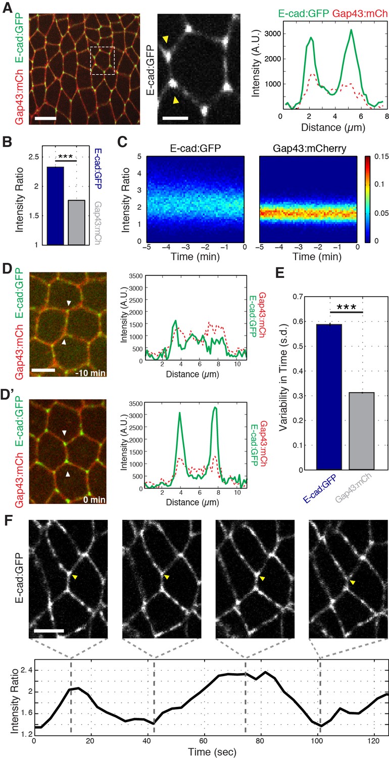
Enrichment and dynamics of E-cadherin at vertices.
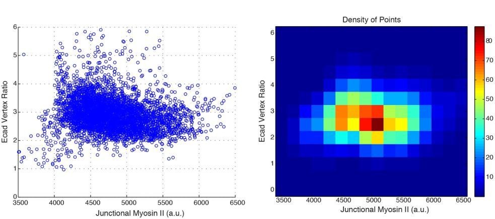
(A) Vertex enrichment of E-cadherin at the initiation of GBE. Endogenous locus E-cad:GFP (green) and plasma membrane marker (Gap43:mCh, red). Single pixel intensity line plot (right) for both E-cad:GFP and Gap43:mCh from region between the yellow arrow heads (middle panel). (B) Vertex:interface intensity ratios computed for each vertex and frame (n = 87662 vertex time points). (C) Heat maps showing the distribution of vertex intensity ratios of Ecad:GFP (left) and Gap43:mCh (right) as a function of time over all embryos aligned to their most contracted state. Color bar shows relative frequency. (D–D’) T1 configuration of cells expressing E-cad:GFP and membrane marker (Gap43:mCh) imaged 10 min before start of GBE (D) and at the onset of intercalation (D’). Intensity line plot corresponds to the single pixel intensity line drawn between the two arrowheads in the left panel. (E) Vertex-associated E-cad intensities display greater variation than control Gap43:mCh membrane marker. Standard deviation over time for a given vertex’s intensity ratio averaged (n = 3188 vertex trajectories). (F) Oscillations in E-cad intensity at an individual T1-associated vertex (yellow arrowhead). The intensity ratio is plotted over time (bottom). Scale bars are 10 µm (A, left), 3 µm (A, middle), and 5 µm (D, F). The data are from five embryos and represent mean ± s.e.m. Statistical tests were done by Student’s t-test. *** denotes p<0.0001.
Figure 1—figure supplement 1
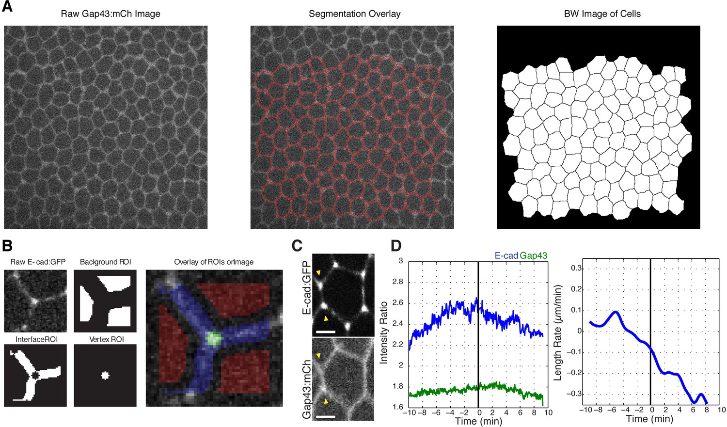
Method of segmentation and vertex analysis showing that vertices become increasingly enriched with E-cadherin prior to the start of cell intercalation.
(A) Images showing a watershed segmentation sample: a raw image in the Gap43:mCh channel (left), raw image with the watershed segmentation lines overlaid in red (middle), and a black and white image of the cell segmented for this frame (right). (B) Images showing the local regions of interest (ROIs) used to measure average background (top middle), interface (bottom left), and vertex (bottom middle) intensities for the vertex shown (top left, raw image). All three ROIs are color shaded on the raw image (right). (C) Image panels showing E-cad:GFP enrichment at vertices (top) and lack of Gap43:mCh enrichment at vertices (bottom); same cell shown in Figure 1A but including Gap43 image. (D) Plot of the average vertex intensity ratios for both E-cadherin and Gap43 taken from 10 min before intercalation starts to 10 min after (left panel), plot of the rate of change of vertical interfaces for the same time period (right panel), n = 580 vertices and n = 61 vertical interfaces. (C) Scale bar is 3 µm.
Figure 2

Radial coupling and sliding of cell vertices during intercalation.
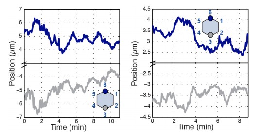
(A) Schematic showing line tension model, in which tensioned springs pull across interface lengths on either side of a contracting interface. Blue and gray dots indicate tricellular vertices. (B) Vertices at either end of a T1 interface display uncoordinated movements and a lack of physical coupling. Vertex displacement plotted over time. (B’) Radial coupling of cell vertices. Vertices that are radially opposed display coordinated movements and coupling of physical displacements. Shaded regions were manually drawn to point out active motion. (C) Quantification of cross-correlation between vertex pairs (n = 385, 772, 769, 1551, 716, 824, 436 for vertex pair categories from left to right, data from first 20 min of cell intercalation when T1 behaviors occur). p<0.0001 for all vertex pairs. Mean ± s.e.m is shown and one sample Student's t-test was performed with hypothesized mean of 0. (D) Total interface lengths (black bar) are conserved during a vertex sliding event, while the contracting L1 interface shrinks (blue). The associated L2 interface (red bar) has a compensatory increase in length as the AP interface contracts (L1, blue bar). Yellow arrowhead shows sliding vertex, white dashed lines mark total length. Scale bar is 5 µm. (E) Total, L1, and L2 lengths plotted over time. (F) Systematic measurement of all fully contracting interface lengths (n = 168 triplet interfaces). Contracting interfaces are aligned and averaged such that their last time point is set to t = 0 (blue curve). The summed lengths of both associated transverse junctions is in red, and the total summed lengths of all three junctions is in black. The data are from five embryos. (G) Time series shows a fully contracting T1 interface (blue), and top (red) and bottom (maroon) transverse junctions lengthening over time. The bottom vertex slides first (yellow arrowhead) followed by the top vertex (white arrowhead). (H) Plot of the interface lengths (same colors in G) and the sum of the three lengths in black; grey shading and black arrowheads point to sliding events.
Figure 3 with 1 supplement
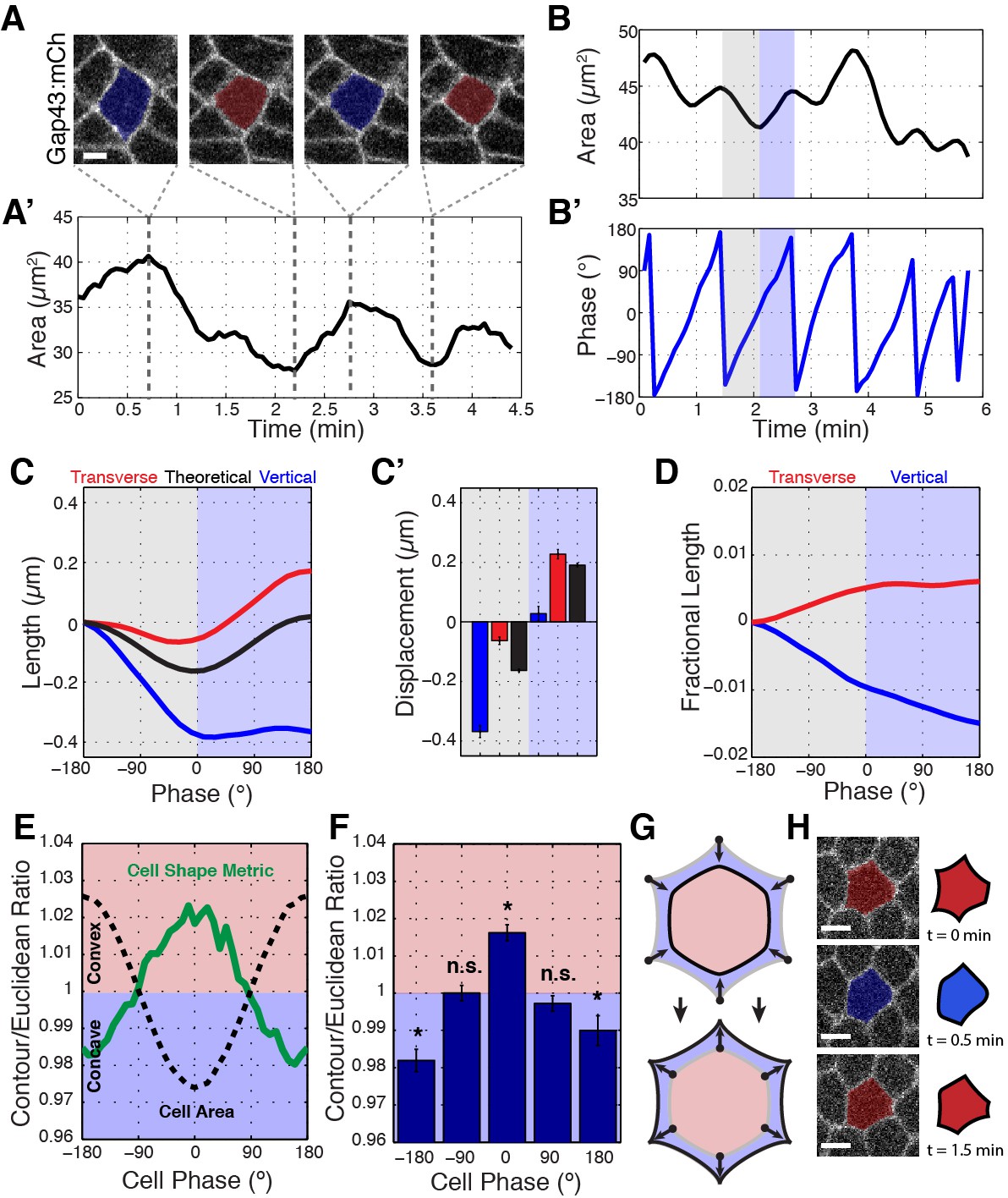
Ratcheted vertex movement is coordinated with changes in apical cell area.
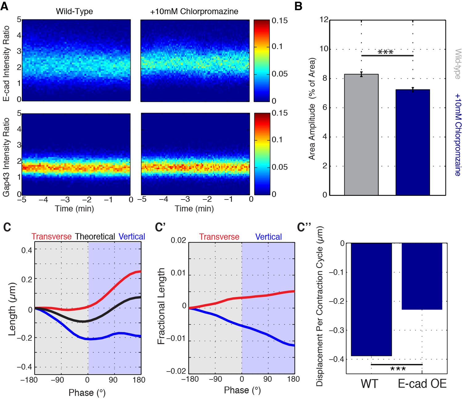
(A–A’) Intercalary cell undergoing apical area oscillations colored blue for maxima and red for minima (A) and plot of the area over time (A’). Gray dashed lines indicate image time points. (B) Plot of cell area trace over time. An oscillatory cycle is highlighted with gray and blue for the decreasing and increasing phases, respectively. (B’) Phasic plot of the cell in (B) with the same highlighted regions shown. (C) Vertical (blue), transverse (red), and theoretical (black) interface length change interpolated into phase space of the associated cell’s area oscillations, n = 212 vertical interfaces. (C’) Quantification of the total length change per decreasing (gray side) and increasing (blue side) half-cycles. (D) Fractional length (Length/Perimeter) change for the same interfaces as analyzed in (C, C’). Vertical interfaces show contraction in fractional length, while transverse interfaces possess compensatory increases in cell length, consistent with vertex sliding. (E) Mean contour over Euclidean cell area ratio (or cell shape metric) verses cell area phase (green curve) and cell area (for reference, black dashed curve), n = 304 cells. (F) Quantification of the cell shape metric at specific phase bins. (G) Illustration showing that cells at area maxima are more concave, while cells at area minima bulge outwards. (H) Sample raw (left) and cartoon (right) cell during one area oscillation. Scale bars are 3 µm (A) and 5 µm (H) and data are from five embryos, the first 20 min of cell intercalation. The data shown in (C’, F) represent mean ±s.e.m. (F) One sample Student's t-test was performed with hypothesized mean of 1. * denotes p<0.01.
Figure 3—figure supplement 1
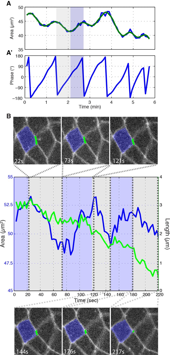
Instantaneous phase of area oscillations and junction ratcheting.
(A, A’) Cell area (A) and phase (A’) plots showing the same data in Figure 3B and B’ except the raw area trace is shown in blue. (B) Plots of a T1 junction length (green) and cell area (blue) of the junction and cell highlighted in the image panels. In the plot area, contraction phases are highlighted in gray and area expansion phases in blue; dashed lines show the time points the images are from. Example taken during first 20 min of intercalation.
Figure 4 with 2 supplements

E-cadherin stabilizes cell vertices.
(A) Example of a cell contracting in area while vertical interfaces contract. Top: Gap43:mCh (plasma membrane) channel with cell color-coded such that darker blue represents smaller apical area. Bottom: yellow arrowhead points to vertex E-cad:GFP that increases as the area contracts and interface length is stabilized at shortened length. White arrowhead shows vertex with less E-cad, where interface length increases during expansion phase following contraction. (B) Cross-correlation of vertex E-cad intensity and cell area rates of change (n = 610 cells). (C) Stabilization of E-cadherin by chlorpromazine injection. Single pixel intensity line plot between the yellow arrowheads shows vertices maintain enrichment of E-cad. (D) Quantification of normalized vertex intensities in control and chlorpromazine-injected embryos for E-cad:GFP (blue) and Gap43:mCh (red) over all vertices and time points in the last 5 min before the most contracted state (control: 87662 vertex time points; chlorpromazine: 60935 vertex time points. (E) Time series of chlorpromazine-injected E-cad:GFP embryo shows vertex (yellow arrowhead) that does not fluctuate in intensity. (F) Averaged standard deviation over time for each vertex’s intensity ratio (n = 3188 control and n = 1934 chlorpromazine vertex trajectories). (G) Length analyses for chlorpromazine injected embryos (n = 219 vertical junctions). Data are from five embryos (control) and three embryos (chlorpromazine) and the first 20 min of cell intercalation. Scale bars are 3 µm. The data shown in (B, D, F, G) represent mean ± s.e.m. Statistical tests were done by Student’s t-test. *** denotes p<0.0001.
Figure 4—figure supplement 1
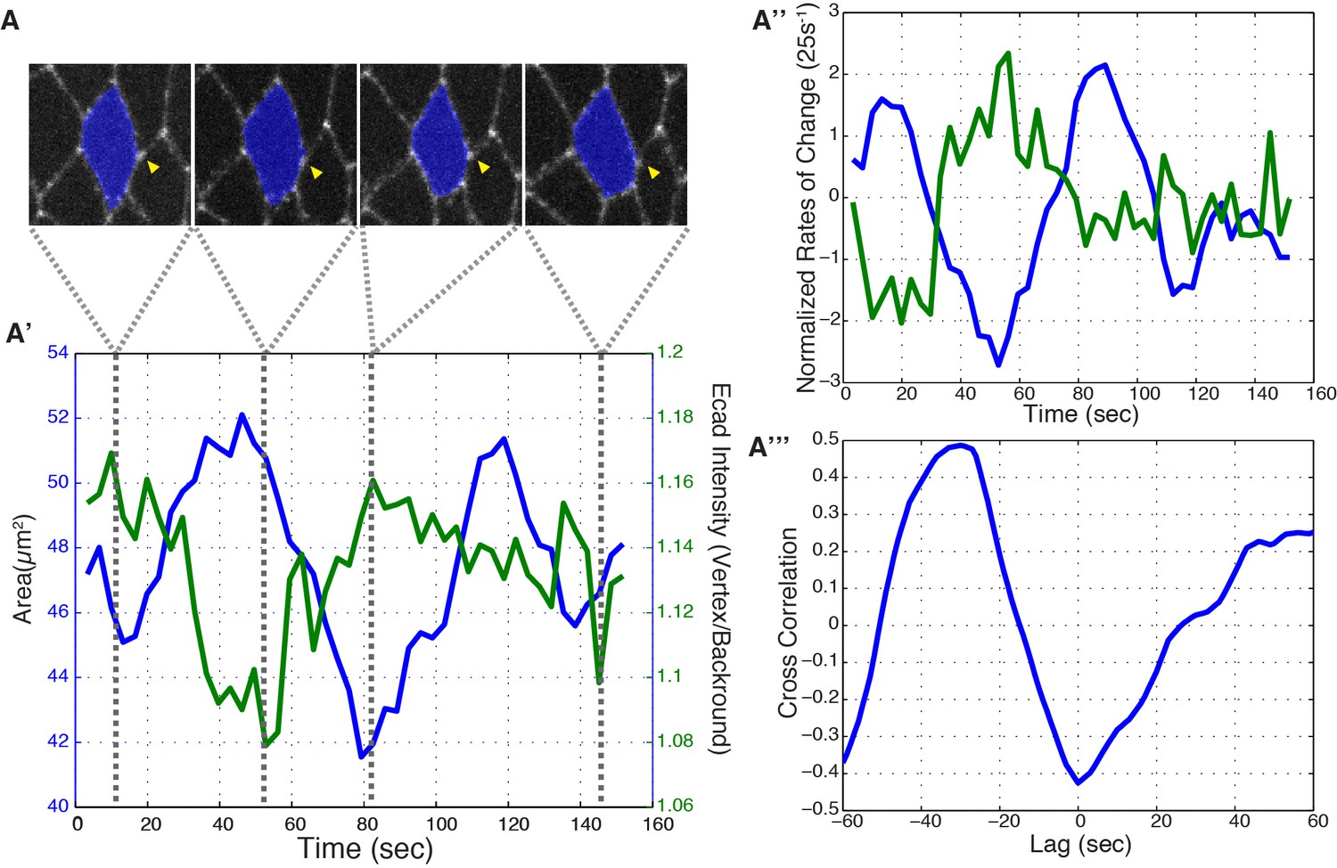
Vertex E-cadherin enrichment is anti-correlated with area oscillations.
(A) E-cad:GFP images at four time points in which enrichment at the vertex (yellow arrowhead) alternates between maxima and minima. (A’) Plot of the vertex intensity ratio for E-cadherin (green) and apical cell area (blue). Dashed lines point to the time points in (A). (A’’) Plot of the rate of change of the intensity ratio and area. (A’’’) Cross-correlation of the rates in (A’’). Example taken during first 20 min of intercalation.
Figure 4—figure supplement 2
Stabilized E-cadherin displays a reduced dynamic range while still possessing oscillations in apical cell area, but junction ratcheting is reduced.
(A) Distribution of intensity ratios for E-cad:GFP (top) and Gap43:mCh (bottom) for wild-type embryos (left column) and chlorpromazine injected embryos (right column). Wild-type distributions are the same as in Figure 1C. Time corresponds to the time until the most contracted time point. (B) Bar graph showing the amplitude of area oscillations as a percentage of the total area in wild-type (n = 540 cells) and Chlorpromazine (n = 364 cells) injected embryos. (C–C’’) Length analysis for Ubiquitin-E-cadherin:GFP; Gap43:mCh embryos (k = 3 embryos, n = 177 vertical interfaces). Mean ± s.e.m are shown in (B, C’) and statistical tests were done by Student’s t-test. *** denotes p<0.0001.
Figure 5 with 1 supplement
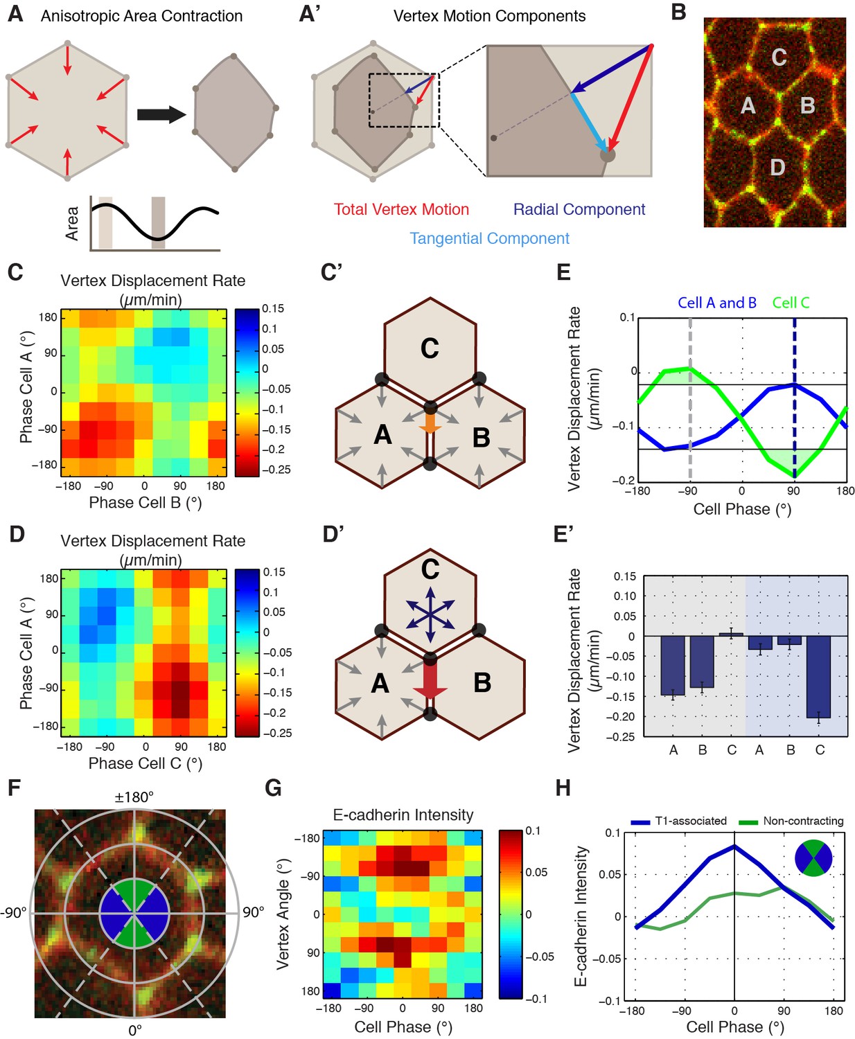
Cell-specific phase anisotropy drives vertex displacements.
(A) Illustration of cell undergoing anisotropic apical area contraction. Red arrows represent inward contractile force. (A’) Illustration of vertex displacement (red arrow) broken into tangential (cyan) and radial (dark blue) motion. (B) Cell labeling scheme: cells A and B share a common vertical, T1 junction, while cells C and D are to the top and bottom of T1-associated vertices, respectively. (C, D) Heat map of the tangential vertex displacement rate with respect to the area phases of cells A and B (C) and cells A and C (D), (n = 171 T1 interfaces from five embryos). (C’, D’) Model schematics showing net displacement of a vertex (orange arrow) when cells A and B are contracting in phase (C’), and a greater net displacement if A and C are in opposite phases with A contracting and C relaxing (D’). (E) Plot of the average rate of tangential vertex displacement for cells A and B (blue) and cell C (green), the black horizontal lines show the max and min levels of cells A and B. (E’) Quantitation of vertex displacement rates at peak contraction and peak expansion (phases ± 90 degrees). Gray and blue shading corresponds to gray and blue dashed lines in (E). (F) Illustration of vertex angle assignment used in (G, H). Ventral direction is assigned as angle zero. Dashed lines separate regions associated with T1 vertices (blue) and non-contracting vertices (green) angle categories. (G) Heat map of the normalized E-cad:GFP intensity of vertices with respect to the angle of the vertex and the cell area phase (n = 238 cells from three embryos). (H) Plot of average normalized E-cad:GFP intensity for T1-associated and non-contracting vertices with respect to area phase. Data are from first 20 min of cell intercalation.
Figure 5—figure supplement 1

Reduced vertex displacements in stabilized E-cadherin embryos.
(A) Heat maps depicting vertex displacement rate (color scale shown on right) against the cell phases of cell A and B (left panel) and cell A and C (right panel) in embryos injected with 10 mM chlorpromazine. Note similar scale of positive (blue) and negative (red) displacements with phase, n = 203 junctions from three embryos, and the first 40 min of intercalation.
Figure 6 with 1 supplement
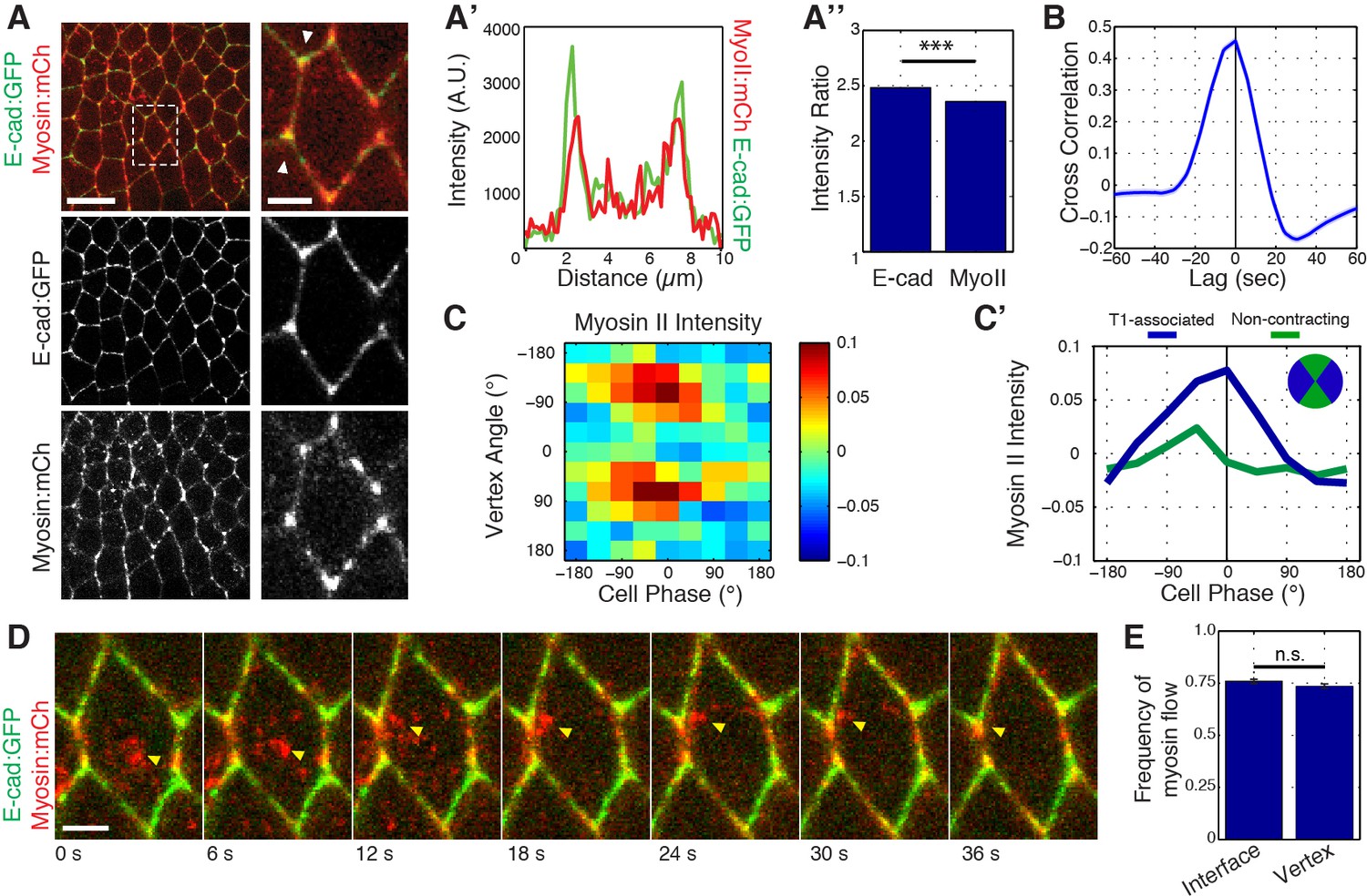
Myosin II dynamics at vertices correlate with, but slightly precede, E-cadherin.
(A) Live imaging of Myosin II (mCh:Sqh, red) and E-cad:GFP (green) embryos during GBE. (A’) Single pixel intensity line plot between arrowheads shown in (a). (A’’) Quantification of Myosin II (mCh:Sqh) and E-cad:GFP vertex intensity ratios (n = 44356 vertex time points). (B) Cross-correlation of the rate of change of intensity ratios for E-cad versus Myosin II (n = 800 vertices). (C) Heat map of the normalized Myosin II vertex intensity with respect to the vertex angle and area phase, n = 238 cells from three embryos. (C’) Plot of average normalized Myosin II intensity for vertical and horizontal vertices with respect to area phase. (D) Time sequence showing medial Myosin II flows (yellow arrowheads) toward vertices in merged images. (E) Quantification of Myosin II (mCh:Sqh) flow destinations. The frequency shows the number of each myosin flow events per cell per min. (n = 30 cells and 537 Myosin II flows in three embryos, n.s., not significant). Data are from three embryos. Scale bars in (A) are 10 µm (left) and 3 µm (right). Scale bar in (D) is 3 µm. *** denotes p<0.0001. Statistical tests were done by Student’s t-test. (A, E) Mean ± s.e.m are shown. Data from first 20 min of cell intercalation.
Figure 6—figure supplement 1
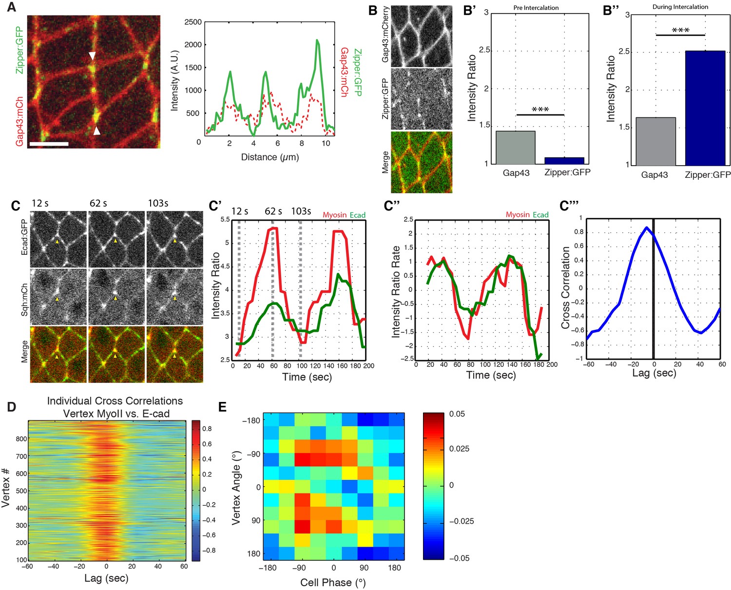
Myosin II localizes to cell vertices with E-cadherin, slightly precedes E-cadherin at the vertices, and is preferentially recruited to vertices associated with AP interfaces.
(A) Embryos expressing endogenously tagged Myosin II heavy chain (Zipper:GFP) and membrane marker Gap43:mCh (left panel). Plot corresponds to the single pixel intensity along the line indicated by the white arrowheads (right panel). (B–B’’) Zipper:GFP (insertion of GFP at endogenous Zipper gene locus) displays vertex enrichment during intercalation. (B) Images in Gap43:mCherry; Zipper:GFP embryos show Myosin II enrichment at vertices. Zipper:GFP is not enriched prior to intercalation (B’, n = 27949 vertex time points from two embryos) and is enriched during intercalation (B’’, n = 57424 vertex time points from two embryos). (C–C’’’) Example images and plots showing the process of cross-correlating E-cadherin and Myosin II at vertices. (C) Images at three time points in which enrichment at the vertex (yellow arrowhead) is at a minimum, maximum, and then minimum. (C’) Plot of the vertex intensity ratio for both E-cadherin and Myosin (mCh:Sqh), dashed lines indicate time points in (C). (C’’) Plot of the rate of change of the intensity ratio in (C’). (C’’’) Cross-correlation of the rates in (C’’). (D) Time resolved cross correlations between vertex Myosin II (mCh:Sqh) and vertex E-cadherin intensity ratios for all individual vertices. These data are averaged in Figure 6B. Note that the peak correlation occurs slightly before the 0 s time lag). (E) Heat map of the normalized Myosin II (Zipper:GFP) vertex intensity with respect to the vertex angle and area phase, n = 245 cells. (B’, B’’) Mean ± s.e.m are shown.
Figure 7 with 1 supplement

Myosin II function is required for E-cadherin dynamics.
(A,B) E-cad:GFP image of cell and single pixel intensity line plot between arrowheads for 100 mM (A) and 25 mM (B) Y-27632 injection. (C,D) Heat map and plot of the normalized E-cad:GFP intensity at vertices with respect to the angle of the vertex and the area phase for 100 mM (c, n = 409 cells) and 25 mM (d, n = 363 cells) Y-27632 injection. (E) Quantification of vertex-to-junction intensity ratios measured for each vertex and each frame of 5 min during GBE (n = 86939 vertex time points). (F) Time sequence of images showing loss of E-cad:GFP dynamics at vertices in 25 mM Y-27832 injected embryos. (G) The averaged standard deviation over time for each vertex’s intensity ratio. Control, n = 3188 vertex trajectories; 25 mM, n = 1868 vertex trajectories. (H, I) Heat map of tangential vertex motion rates versus the phases of cell A and cell B (left) and cell A and cell C (right) for 25 mM (H) and 100 mM (I) Y-27632 injection. (H) n = 175 junctions. (I) n = 220 junctions. (J) Model for vertex-directed changes in cell topologies. As a cell adjacent to a vertex along the AP axis contracts (gray arrows), and the adjacent cell along the DV axis expands (blue arrows), the vertex experiences a cumulative asymmetric force, causing it to slide along the interface (middle row, cyan line). At the molecular level, medial Myosin II flows consolidate E-cadherin at cell vertices post-vertex sliding, resulting in a local increase in adhesive stability. This is coordinated with oscillations in apical cell area, which ensures progressive, non-reversible vertex displacements (bottom). Gray shading indicates a contractile phase; blue indicates expansion. Control data from three embryos, Y-27632 25 mM from three embryos, and Y-27632 100 mM from three embryos. Scale bars are 3 µm. *** denotes p<0.0001. (E, G) Mean ± s.e.m are shown. Data from first 20 min of cell intercalation.
Figure 7—figure supplement 1
E-cadherin vertex enrichment is lost in sqhAX mutant embryos and area oscillation amplitude is reduced under Y-27632 treatment.
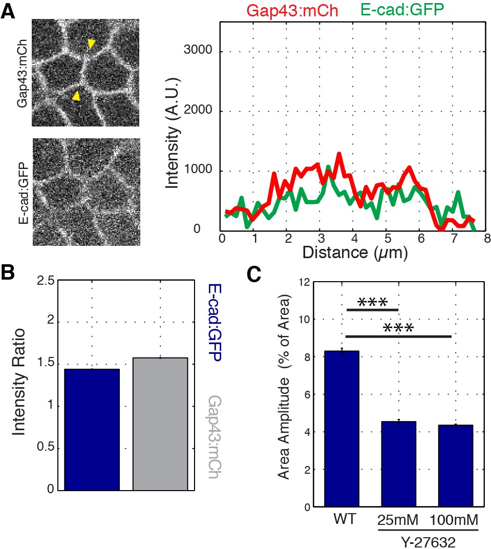
(A) sqhAX mutant embryos expressing E-cad:GFP and membrane marker Gap43:mCh. sqh encodes the regulatory light chain of Myosin II in Drosophila. Plot corresponds to the single pixel intensity along the line indicated by the yellow arrowheads (right panel). As expected, the sqhAX vertex phenotype is partially penetrant (42%). (B) Vertex intensity ratio quantified in sqhAX mutant embryos (k = 2 embryos, n = 6704 vertex time points over the first 20 min of cell intercalation). (C) Bar graph showing the amplitude of area oscillations as a percentage of the total area in wild-type (n = 540 cells) and Y-27632 (n = 407 cells for 100 mM, n = 362 cells for 25 mM) injected embryos (concentrations are noted in graph). Mean ± s.e.m are shown and statistical tests were done by Student’s t-test. *** denotes p<0.0001.
Author Response Image 1
Author response image 2

Author response image 3
Author response image 4
Videos
Video 1
E-cadherin intensity ratio of vertices are dynamic.
Time-lapse images of an embryo expressing the adhesion marker E-cad:GFP during germband extension. The vertex (marked by yellow arrow) exhibits dynamic changes in E-cadherin enrichment. The intensity ratio is plotted as a function of time (bottom). Total time is 125 s, 30 frames/second. Scale bar is three microns.
Video 2
Contracting vertices slide along cell interfaces.
Time-lapse images of an embryo expressing the membrane marker Gap43:mCherry during germband extension. A single vertex can move independently of adjacent vertices and interfaces to result in the cell-shape changes associated with T1 contraction. Anterior is left, ventral is down. Total time is 118.8 s, 25 frames/second. Scale bar is three microns.
Video 3
Cell area oscillations during germband extension.
Time-lapse images of a cell (shaded blue) expressing the membrane marker Gap43:mCherry undergoing area oscillations (top) and a plot of the cell area (bottom) over time. Total time is 264 s, 45 frames/second. Scale bar is three microns.
Video 4
Cell area oscillations in chlorpromazine injected embryo.
Time-lapse images of a cell (shaded blue) expressing the adhesion marker E-cad:GFP undergoing area oscillations (top) and a plot of the cell area (bottom) over time. Total time is 151.8 s, 45 frames/second. Scale bar is three microns.
Video 5
Myosin II flows toward vertices.
Time-lapse images of an embryo expressing E-cad:GFP and mCherry:Myosin II. Myosin II from the medial/apical region of the cell flows toward a vertex, resulting in Myosin II vertex enrichment. Anterior is left, ventral is down. Total time is 48.8 s, 10 frames/second. Scale bar is five microns.
Additional files
-
Transparent reporting form
- https://doi.org/10.7554/eLife.34586.022
Download links
A two-part list of links to download the article, or parts of the article, in various formats.
Downloads (link to download the article as PDF)
Open citations (links to open the citations from this article in various online reference manager services)
Cite this article (links to download the citations from this article in formats compatible with various reference manager tools)
Vertex sliding drives intercalation by radial coupling of adhesion and actomyosin networks during Drosophila germband extension
eLife 7:e34586.
https://doi.org/10.7554/eLife.34586


