Causal contribution and dynamical encoding in the striatum during evidence accumulation
- Princeton Neuroscience Institute, United States
- Helen Wills Neuroscience Institute, United States
- University of California, Davis, United States
- Howard Hughes Medical Institute, United States
Figures
Figure 1 with 2 supplements
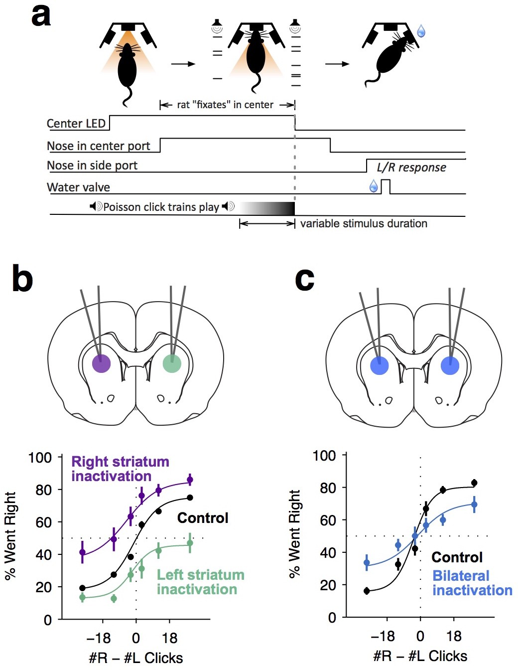
Dorsal anterior striatum is required for unimpaired performance on the Poisson-clicks evidence accumulation task.
(a) Sequence of events in each trial of the rat auditory Poisson-clicks task. From left to right: after light onset above the center port, rats 'fixate' their position by placing their nose inside the center port. During nose-fixation, two different trains of randomly timed auditory clicks are played concurrently from the left and right speakers. Upon termination of the sound trains, the light above the center port turns off and the rat needs to make a choice, poking into the left or right port to indicate if more clicks were played on the left or right sides, respectively. (b) Unilateral infusion of muscimol into the striatum results in a significant ipsilateral bias on accumulation trials. Purple and cyan psychometric curves show data on days of right and left striatal infusions (n left sessions = 29; n right sessions = 29), respectively. Black psychometric curve shows data from control sessions that occurred one day before infusion sessions (n = 58). (c) Bilateral infusion of muscimol into the striatum results in significant impairment on accumulation trials. The blue psychometric curve is from bilateral infusion sessions (n = 26) and the black psychometric curve is from control sessions that occurred one day before bilateral infusion sessions (n = 26). Data are shown as mean ± S.E.M.
Figure 1—figure supplement 1

Rat behavior indicates the accumulation of auditory evidence over the entire trial.
(a) Averaged psychometric curve showing average performance across all rats during the Poisson-clicks task (n = 20 rats). (b) Chronometric curve of the same rats showing improved performance with longer stimulus durations. Difficulty is grouped by the ratio of auditory clicks played on the left and right sides. (c) Psychophysical reverse correlation analysis (Brunton et al., 2013). Red and green curves correspond to trials in which rats went right and left, respectively. Note the stability of each curve, indicating that pieces of sensory evidence (auditory clicks) throughout the trial were weighted evenly in the rats’ decision process. This result is further corroborated by the long accumulation time constants exhibited by the rats (see Supplementary file 1).
Figure 1—figure supplement 2
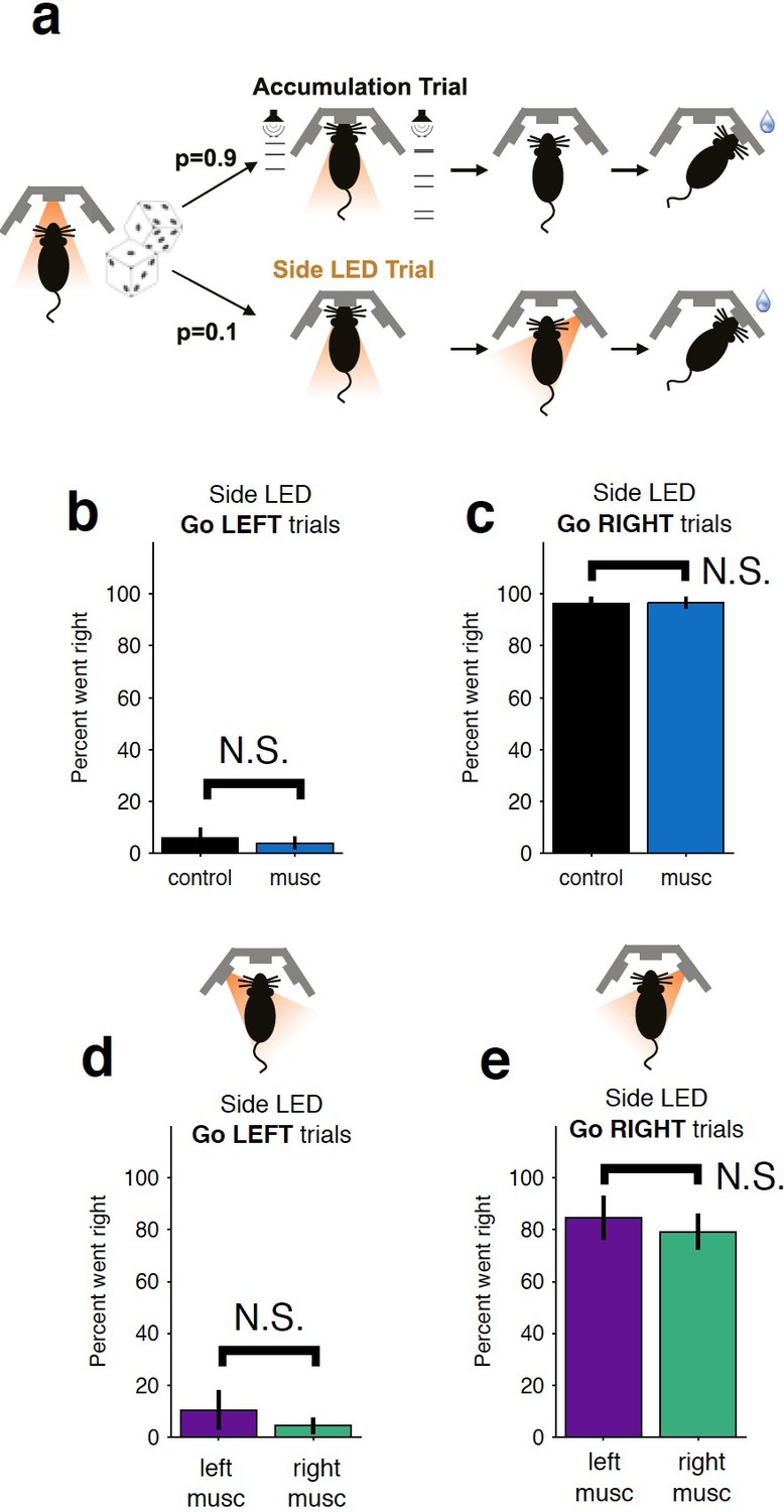
Control LED trials indicate that the behavioral bias and impairments resulting from striatal inactivation are not due to motor impairments.
(a) On ~10% of trials, rats were presented with an LED above the right or left port and had to orient towards that port. Thus, they had to perform the same motor action but success was not dependent on evidence accumulation. No significant impairment is observed for either bilateral inactivation (b–c) or unilateral (d–e) inactivations. The color scheme is the same as that used in Figure 1b–c. musc, muscimol.
Figure 2 with 4 supplements
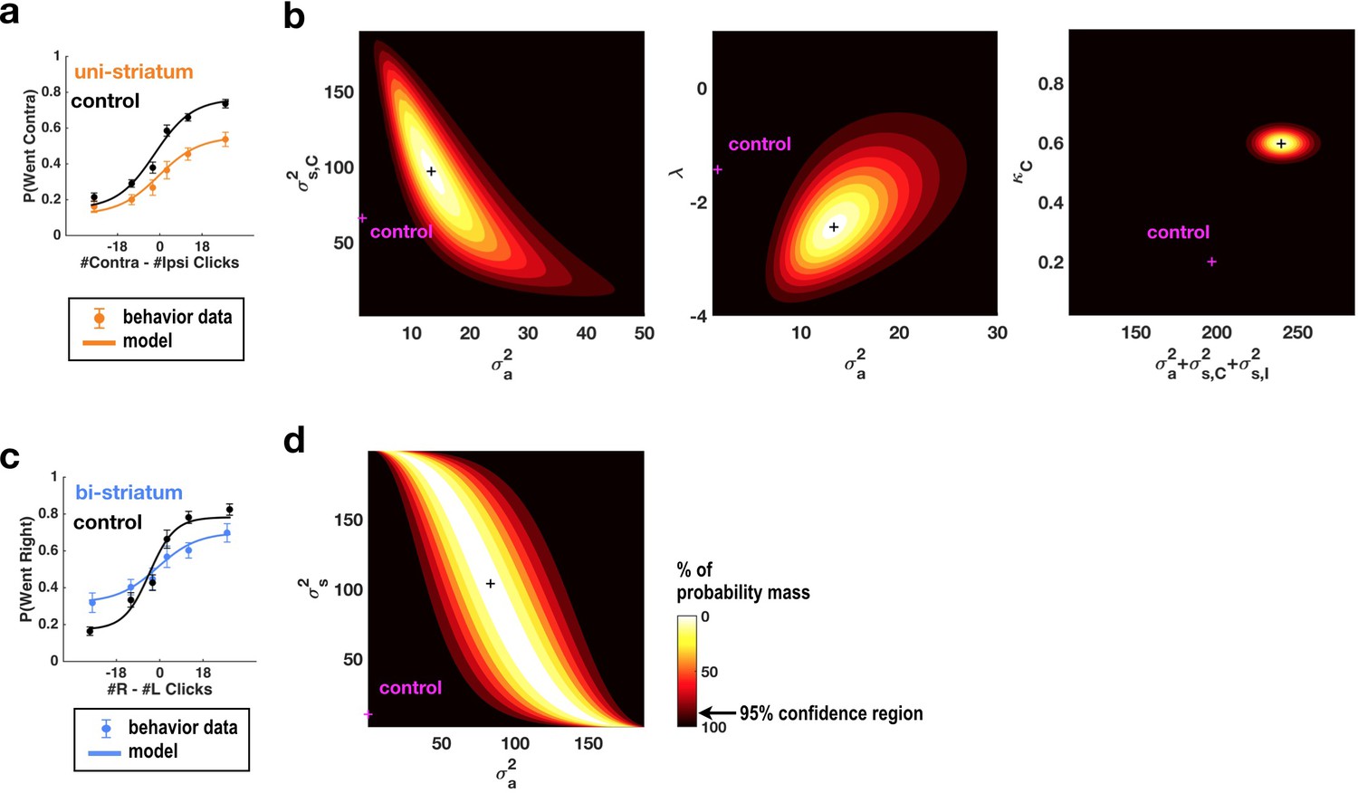
Fits of the model of Brunton et al. (2013) and Erlich et al. (2015) to data from sessions following muscimol inactivation of the striatum.
(a) Psychometric curves for control and unilateral inactivation data. Left and right inactivations were collapsed together. Orange data points are from sessions following unilateral infusions of muscimol. The black and orange lines are the psychometric curves predicted from the model fit to the control and inactivation data, respectively. (b) Normalized likelihood of the data given the model, shown as a function of the parameters for which best-fit values for inactivation data were significantly different from best-fit values for control data. Magenta shows the best-fit values for control datas. The black cross shows the best-fit values for inactivation data. The color scale indicates the percentage of probability mass; the region of probability mass >95 indicates the 95% confidence region. Left: sensory noise for the side contralateral to the infusion versus accumulator noise. Although there is a trade-off between accumulator and sensory noise, the weighted sum of the accumulator and biased sensory noise has a best-fit value following unilateral inactivations that is significantly greater than its control best-fit value. Middle: leak/instability parameter versus accumulator noise. Right: summed sensory plus accumulator noise versus lapse rate, which shows that in fact the lapse rate κC does not trade off with the summed noise. (c,d) As in panels (a,b) but for bilateral striatum inactivation data, and for a model where the sensory noise is constrained to be the same for both sides of the brain, so there is only one sensory noise parameter. Here the tradeoff between sensory noise and accumulator noise is large enough that we cannot distinguish whether one or both are significantly different from their control values, but there is nevertheless a significant increase in their sum.
Figure 2—figure supplement 1

Confidence regions with unbounded parameter optimization.
When a parameter θ is bounded, we transfer with monotonic function f. is unbounded in infinite space, but is constrained in the desired range for . The optimization on finds the optimal and confidence region (95% confidence ellipse) in infinite space (middle column). The optimal and confidence region are transformed to the original coordinates (regular space) with function f (left column). To compare control and inactivation distribution, we subtracted two Gaussian distributions and tested the distance from the origin (red cross), showing that the two distributions are significantly different (right column). (a) Confidence regions for unilateral inactivation and control data. Orange solid lines indicate 95% confidence regions for inactivation data, and black solid lines indicate 95% confidence regions for control. Top row: σa vs. σs,C. Middle row: σa vs. λ. Bottom row: summed noise vs. κC. Elongated ellipses oriented diagonally indicate that parameters can trade off with each other (e.g., σa vs. σs,C). An example of parameters that do not trade off is lapse rates versus noise parameters (summed noise vs. κC). (b) Confidence regions for unilateral inactivation and control data. Blue solid lines indicate 95% confidence regions for inactivation data, and black solid lines 95% confidence regions for control.
Figure 2—figure supplement 2
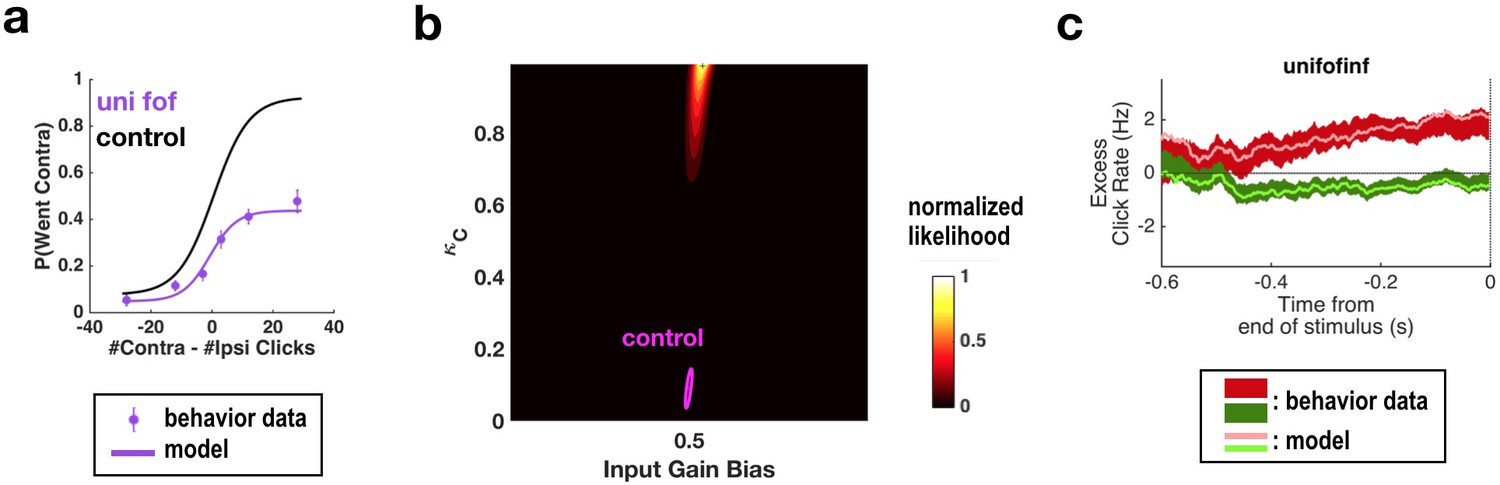
Fitting all parameters simultaneously for unilateral FOF inactivation data confirms the conclusions found by fitting only two parameters at a time.
(a) Psychometric curves for control and unilateral FOF inactivation data. The black line is the model fit to the control data. The purple circles with error bars are experimental data from unilateral FOF inactivation sessions, and indicate fraction of Contra choice trials (mean ± binomial 95% confidence interval) across trial groups, with different groups having different #Contra − #Ipsi clicks. The purple line is the psychometric curve generated by the post-categorization bias model. (b) The two-dimensional normalized likelihood surface. The peak of the likelihood surface for the inactivation data is significantly different from that for the control data for post-categorization bias (from 0.0895 to 0.9857). Input gain bias (which is parametrized so that 0.5 means no side bias) is not significantly different from its control value. (c) Reverse correlation analyses showing the relative contributions of clicks throughout the stimulus in the rats’ decision process. The thick dark red and green lines are the means ± standard error across trials for contralateral and ipsilateral trials. Thin light red and green lines are the reverse correlation traces generated by extended model.
Figure 2—figure supplement 3
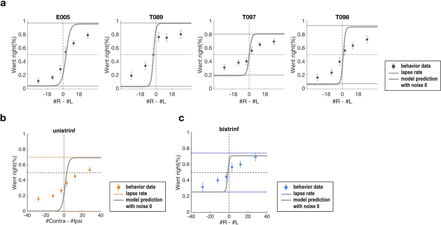
Psychometric curves of data and simulation data for which sensory and accumulator noise parameters are set to zero.
(a) Simulation results using the best-fit parameters for control data in unilateral inactivation experiments (Supplementary file 1), but with noise parameters set to zero. The solid lines (model prediction) reach the lapse parameter values (dotted line, Supplementary file 1). (b) Same format as (a), for best-fit parameter values for unilateral inactivation data Supplementary file 2). (c) Same format as (a), for best-fit parameter values for bilateral inactivation data (Supplementary file 3). These panels show that the noise parameters largely account for the errors observed with the strongest stimuli.
Figure 2—figure supplement 4
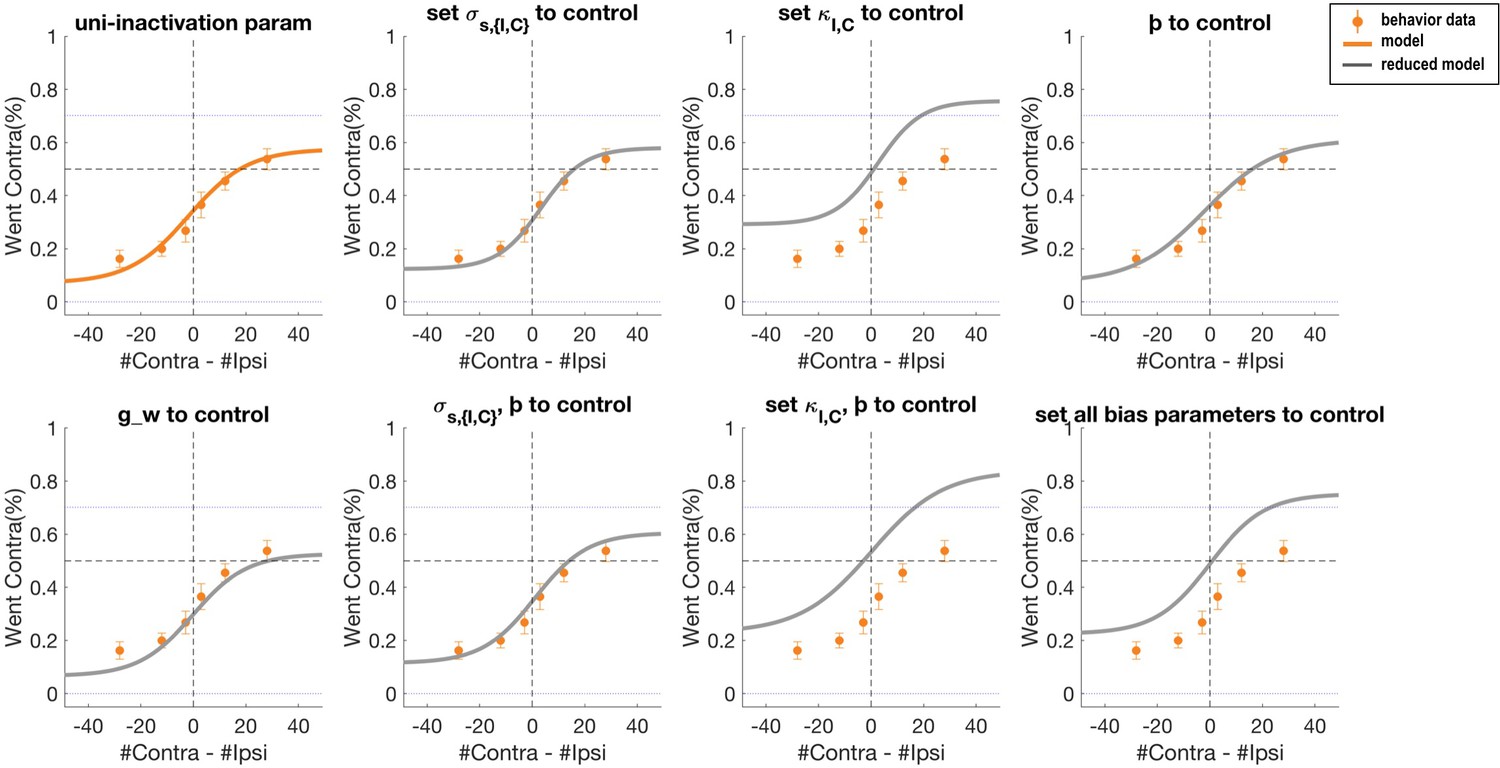
Psychometric curves of data and simulation data for which the bias parameters are adjusted to control best-fit parameter values in the 11-parameter model.
Orange dots and error bars show the unilateral striatum inactivation data. The orange solid line is the model prediction obtained with the 11-parameter full model. The grey solid line is the model prediction when each bias parameter is set to the corresponding control parameter value.
Figure 3 with 1 supplement
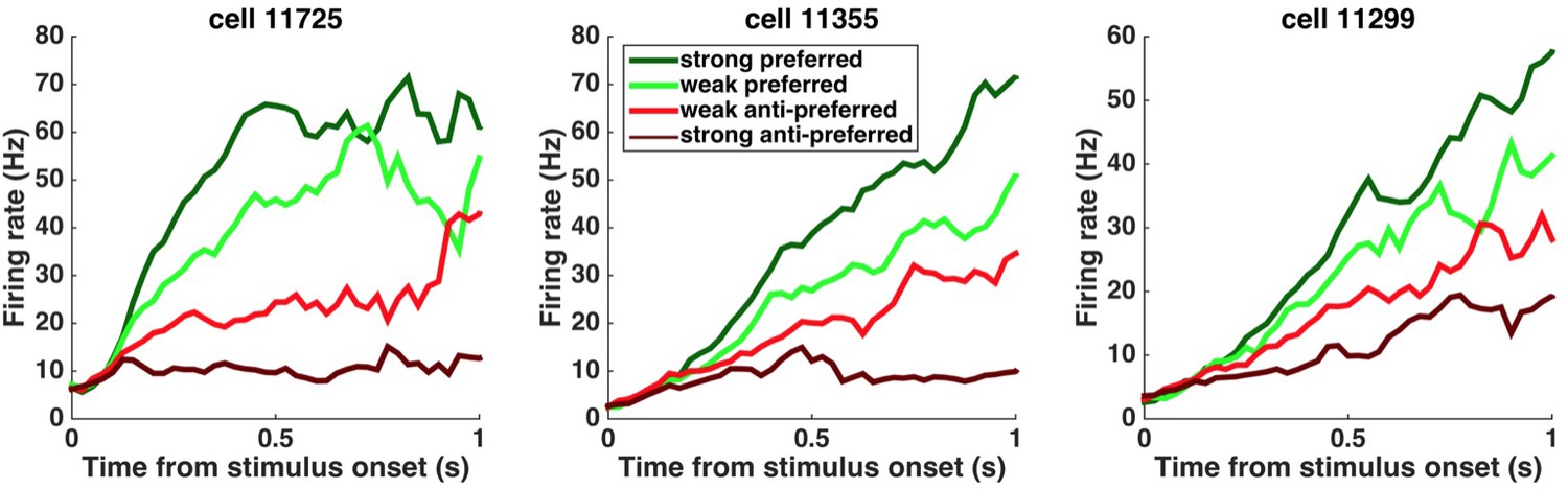
Peri-stimulus time histograms (PSTHs) of example neurons.
PSTHs aligned to stimulus onset are shown for three example striatum neurons. Trials were sorted into four stimulus-strength bins for each neuron. Green traces correspond to the preferred-direction stimuli and red traces to anti-preferred-direction stimuli. Darker colors correspond to stronger stimuli (less difficult) and brighter colors correspond to weaker stimuli (more difficult).
Figure 3—figure supplement 1
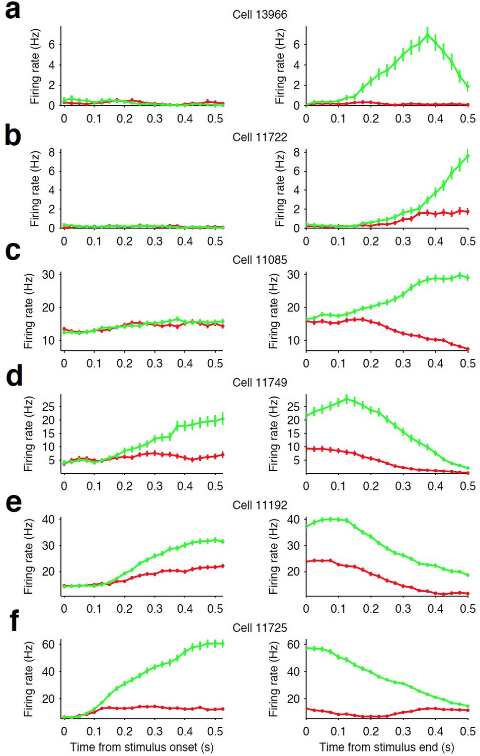
Firing rate modulation of striatal neurons.
(a–c) Examples of three striatal neurons that did not exhibit significant modulation in their firing rates during stimulus presentation (left column) but did show movement-related firing rate modulation (right column). (d–e) Examples of three striatal neurons that exhibited modulation of their firing rate during stimulus presentation and exhibited side-selective responses. This latter class of neurons are the subject of our analyses in this manuscript. For all examples, green traces are the response for preferred direction choices and red for non-preferred direction choices (see Materials and methods).
Figure 4 with 1 supplement
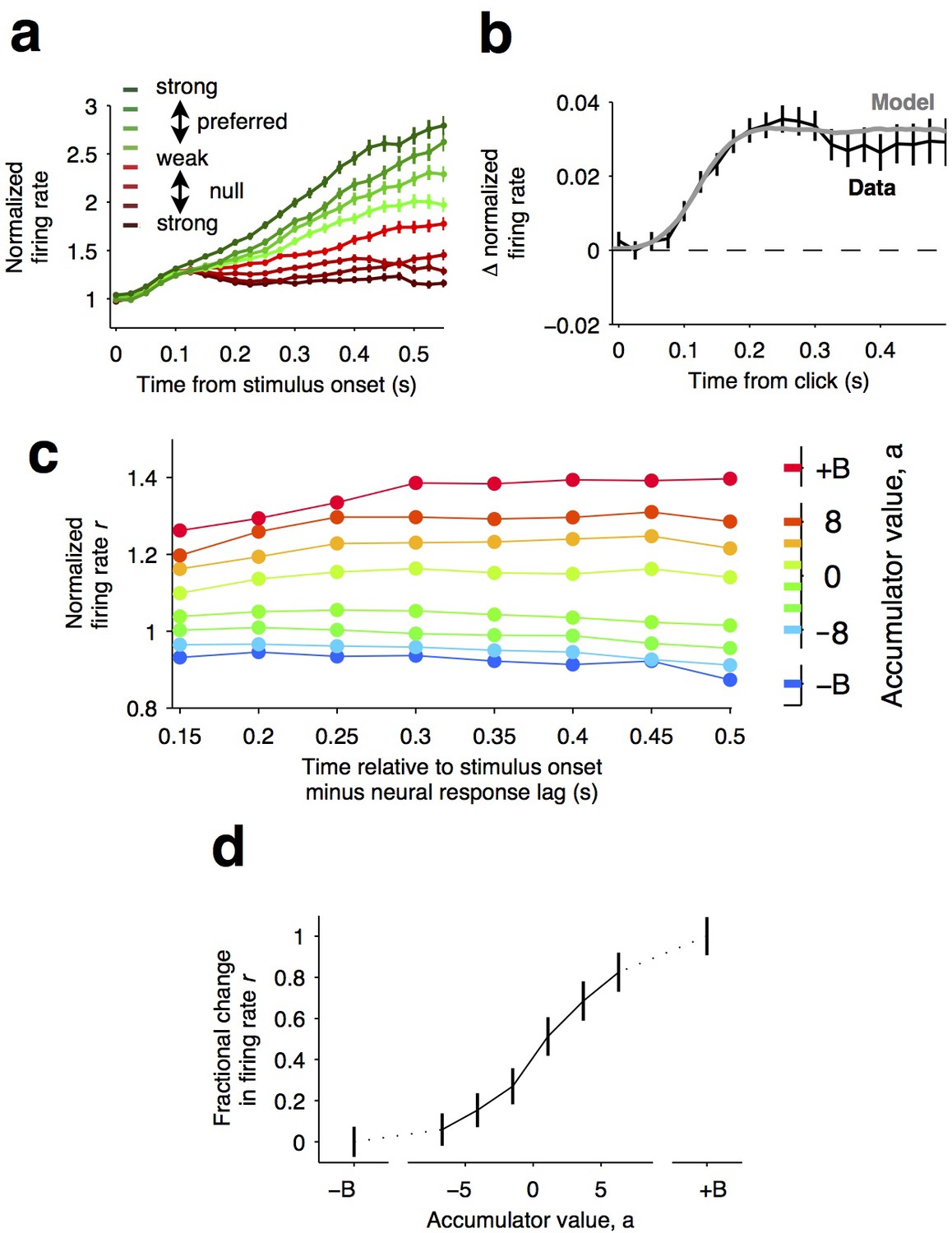
Graded representation of accumulated evidence in the dorsal striatum.
(a) Responses of pre-movement side-selective striatal neurons during evidence accumulation (mean ± S.E.M.). Trials are grouped by the average strength of sensory evidence with greener and redder colors corresponding to stimuli in the preferred and non-preferred direction of the neurons, respectively. Each group of trials is sorted on the basis of the difficulty of the trials from easy to hard, corresponding to darker and lighter colors, respectively. Note the significant dependence of ramping responses on stimulus strength (n = 64 neurons from three rats). (b) Click-triggered average response ± S.E.M. Note the close correspondence of the average click-triggered population response to a theoretical prediction of a fixed-magnitude and sustained increase in the neurons’ firing rate (see Materials and methods). (c) Firing of striatal neurons aligned to trial onset minus the neural response lag (150 ms; see Materials and methods) grouped on the basis of model-derived accumulator value (colors with ± B correspond to sticky accumulation bounds). Note that this accumulator value to firing rate map is graded and fairly stable over time (n = 64 neurons). (d) The population change in firing rate as a function of accumulator value averaged across time exhibits a graded response.
Figure 4—figure supplement 1
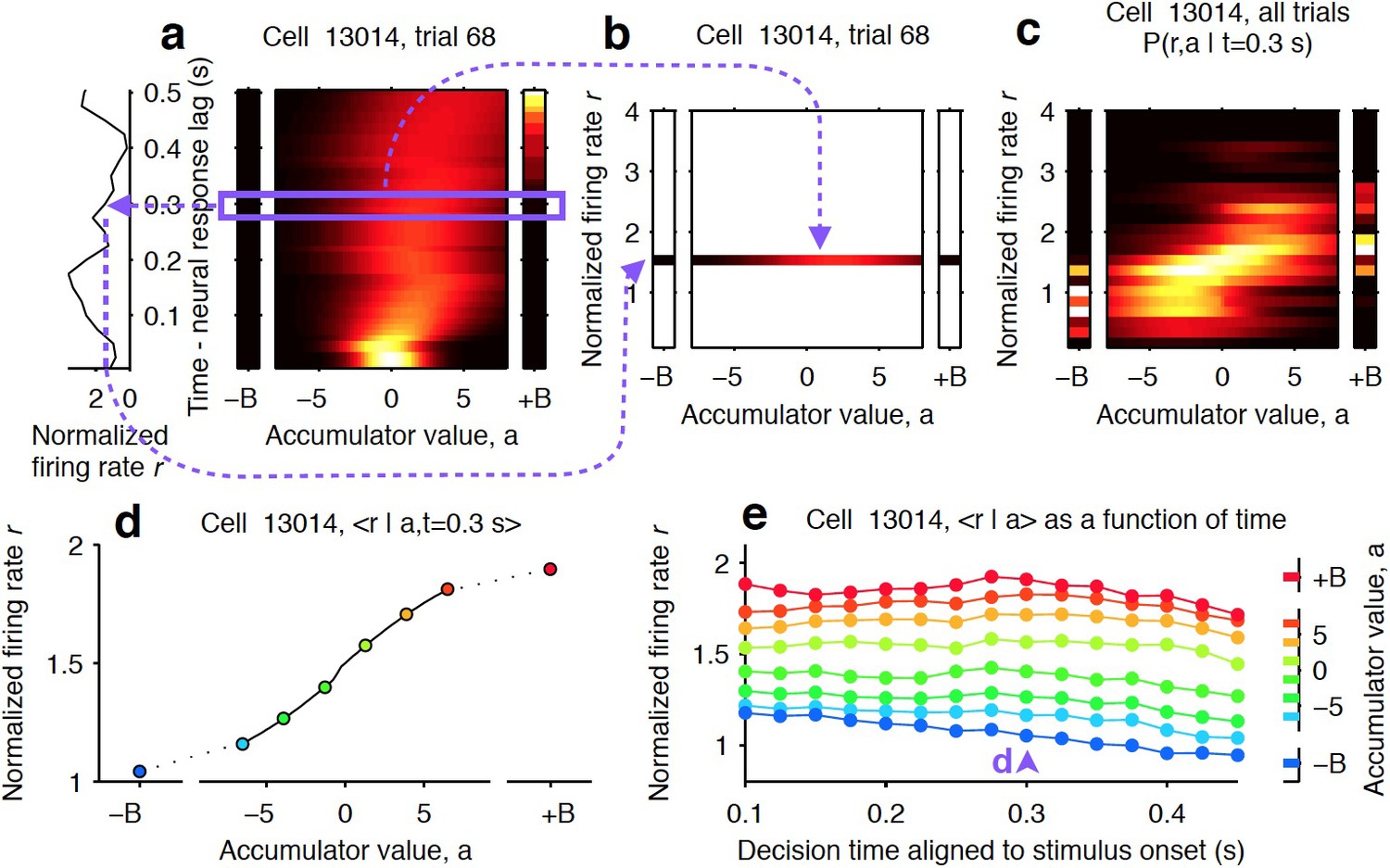
Computing tuning curves that describe the relationship between neural activity and accumulated evidence.
(a) One trial for an example neuron from the striatum. The left side shows the firing rate of the neuron, and the right side shows the behavioral model’s estimate of the evolution of the distribution of the accumulator value, a. The heat map illustrates the temporal evolution of a probability distribution over possible values of the decision variable (see Materials and methods). Time runs vertically and is aligned to stimulus onset minus neural response lag (see Materials and methods). ± B correspond to the ‘sticky’ decision-commitment bounds on evidence accumulation. (b) Building a map of firing rate versus accumulator value. At a given time point (here, t = 0.3 s), we copy the distribution of the accumulator value (blue box) to a vertical position given by the firing rate of the neuron. (c) Continuing with the same time point, we add a slice from every recorded trial. Thus, the full distribution of accumulator values for each trial contributes to the estimate for each firing rate bin. This produces the full joint distribution P(r,a | t = 0.3), the probability of seeing firing rate r and accumulator value a at time t = 0.3 s. (d) The accumulator values are binned, and the mean firing rate is computed for each bin to generate a neural tuning curve as a function of the accumulator value. (e) The process is repeated for each time point. Each vertical slice corresponds to a tuning curve, with that from (d) shown above the blue arrowhead.
Figure 5
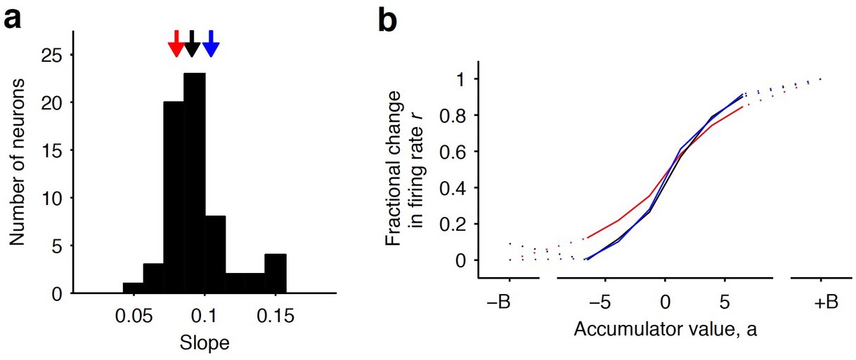
Distribution of tuning curve slopes for individual striatal neurons.
(a) Histogram of the slope of individual neurons obtained from a sigmoidal fit of the relationship between firing rate and accumulator value. The black arrow indicates the median value of the distribution (50th percentile). Red and blue arrows indicate points corresponding to the 20th and 80th percentile marks, respectively. (b) Example tuning curves shown for 20th, 50th, and 80th (colored as in [a]) percentile neurons. Graded encodings of accumulated evidence are exhibited for all of these neurons.
Figure 6
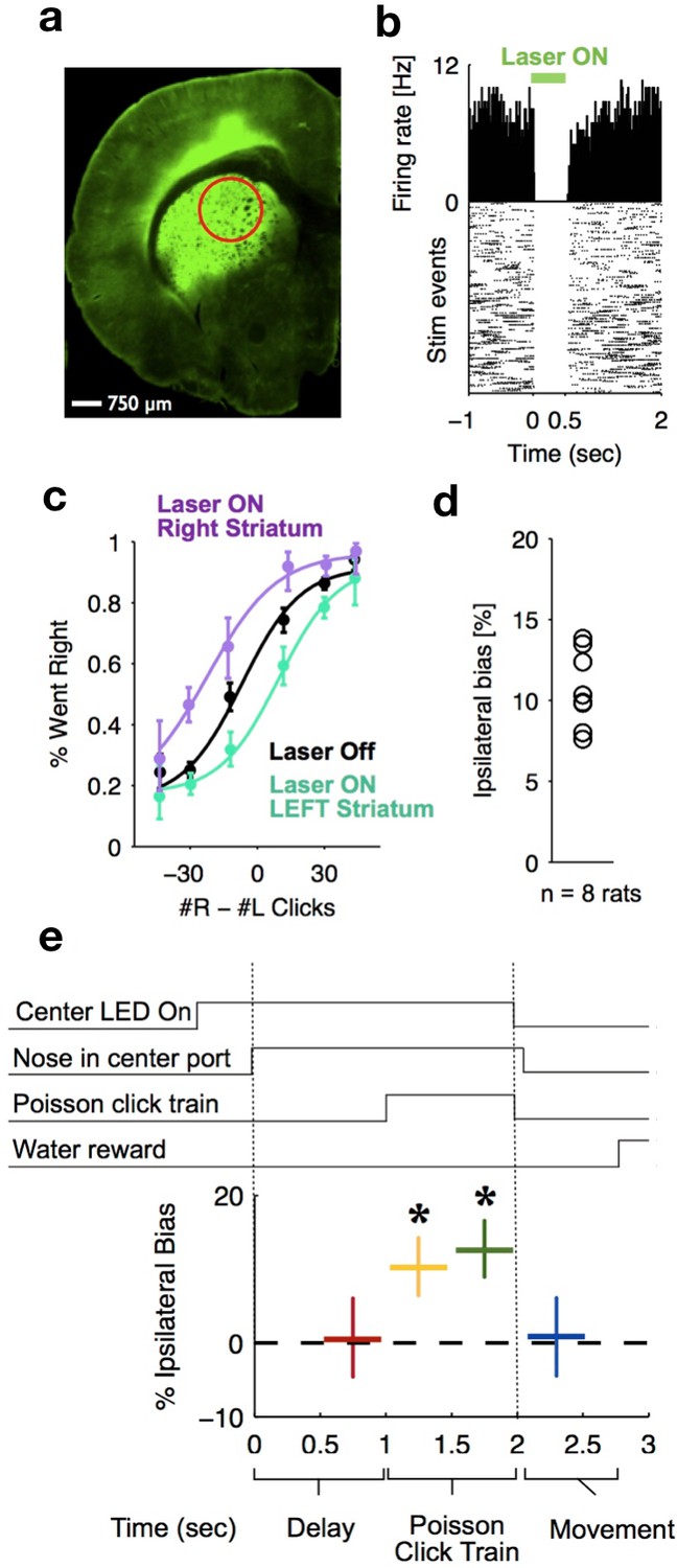
Optogenetic inactivation reveals that dorsal striatal activity causally contributes to decision formation throughout the accumulation process but not before nor after.
(a) Coronal section of the left hemisphere showing the expression of eYFP-eNpHR3.0 in the left dorsal striatum. Optical fiber localization and 750 μm estimated inactivation radius are indicated by the red circle. (b) Raster plot (bottom) and peri-stimulus time histogram (top) showing the effectiveness in silencing of local striatal activity in response to delivery of green light (indicated by the green bar at the top). (c) Unilateral full-trial optical inactivation of the striatum results in an ipsilateral bias in accumulation trials. The purple and cyan psychometric curves show data for right and left striatal inactivation, respectively, whereas the black psychometric curve shows data from control trials that occurred on the same days (n = 8 rats). (d) Scatter plot indicated the mean ipsilateral bias for each individual rat. (e) Bottom: behavioral bias caused by 500 ms inactivation during the pre-stimulus delay period (red), the first half of the sensory stimulus (yellow), the second half of the stimulus (green) and upon initiation of movement (blue). Top: task structure. Note the significant effect (indicated by an asterisk) only during evidence accumulation but not prior to the presentation of sensory stimuli nor after.
Figure 7

Comparison of early stimulus period optogenetic inactivation effects in the striatum and frontal orienting field (FOF).
Optogenetic inactivation of the anterior dorsal striatum during the first half of the 1 s stimulus presentation period produced a significantly larger effect than the same manipulation of the FOF (p<0.01), with the latter data coming from a previous report. For this analysis, individual trials were resampled with replacement from both data sets across 1000 iterations, and the difference in inactivation effect was calculated for each iteration to provide a nonparametric statistical comparison. As reported above, the first-half anterior dorsal striatum effect itself is significant, and as reported previously, the first-half FOF effect is not significant, but a direct comparison as described here is still necessary to establish a significant difference.
Additional files
-
Supplementary file 1
Best-fit parameters.
This table shows the values of the parameters that maximize the likelihood of the eight-parameter accumulator model for all no-perturbation sessions of each rat (four rats for pharmacological inactivation study, three rats for electrophysiology, and 13 rats for optogenetics). The 95% confidence range is shown in brackets underneath each estimate.
- https://doi.org/10.7554/eLife.34929.017
-
Supplementary file 2
Best fit parameters (unilateral striatum inactivation data, n = 4 rats).
Table 2 shows the values of the parameters that maximize the likelihood of the 11-parameter accumulator model for unilateral striatum inactivation data (n = 3528 trials) and unilateral striatum control data (n = 8349 trials). The 95% confidence range is shown in brackets underneath each estimate. The control corresponds to data taken on the no-infusion days immediately prior to the infusion day. Infusion sessions were spaced apart from each other by at least, and often more, non-infusion days.
- https://doi.org/10.7554/eLife.34929.018
-
Supplementary file 3
Best fit parameters (bilateral striatum inactivation data, n = 3 rats).
Table3 shows the values of the parameters which maximize the likelihood of the 8-parameter accumulator model for the bilateral striatum inactivation data (n = 2266 trials), the fit to the bilateral striatum control data (n = 3846 trials). 95% confidence range is shown in brackets underneath each estimate. Control corresponds to data taken on the no-infusion days immediately prior to the infusion day. Infusion sessions were spaced apart from each other by at least seven, and often more, non-infusion days.
- https://doi.org/10.7554/eLife.34929.019
-
Supplementary file 4
Best fit parameters (unilateral FOF inactivation data, n = 10 rats).
Table 4 shows the values of the parameters that maximize the likelihood of the 11-parameter accumulator model for the unilateral FOF inactivation data (n = 3836 trials), and the fit to the unilateral FOF control data (n = 47,580, trials). The 95% confidence range is shown in brackets underneath each estimate. The control corresponds to data taken on the no-infusion days immediately prior to the infusion day. Infusion sessions were spaced apart from each other by at least seven, and often more, non-infusion days.
- https://doi.org/10.7554/eLife.34929.020
-
Supplementary file 5
Best fit parameters (unilateral striatum inactivation data, n = 4 rats).
Table 5 shows the values of the parameters that maximize the likelihood of the eight-parameter accumulator model for the unilateral striatum inactivation data (n = 1809 trials) and bilateral FOF control data (n = 1531 trials). The 95% confidence range is shown in brackets underneath each estimate. The control corresponds to data taken on the no-infusion days immediately prior to the infusion day. Infusion sessions were spaced apart from each other by at least seven, and often more, non-infusion days.
- https://doi.org/10.7554/eLife.34929.021
-
Supplementary file 6
BIC – 11 p full model (unilateral inactivation).
Table 6 shows, for each parameter, the difference in Bayesian Information Criterion (BIC; Nagin, 1999) for the 11-parameter full model, minus the BIC for the model with that parameter removed. Positive numbers thus favor keeping the parameter. Calculations are for data for unilateral striatum inactivations (n = 3528 trials) and the corresponding control data (n = 8349 trials).
- https://doi.org/10.7554/eLife.34929.022
-
Supplementary file 7
BIC – 8 p full model (bilateral inactivation).
Table 7 uses the same conventions and shows, for each parameter, the difference in BICs for the eight-parameter full model minus a model with that parameter removed. Calculations are for data from bilateral striatum inactivations (n = 2266 trials) and for corresponding control data (n = 3846 trials).
- https://doi.org/10.7554/eLife.34929.023
-
Transparent reporting form
- https://doi.org/10.7554/eLife.34929.024
Download links
A two-part list of links to download the article, or parts of the article, in various formats.
Downloads (link to download the article as PDF)
Open citations (links to open the citations from this article in various online reference manager services)
Cite this article (links to download the citations from this article in formats compatible with various reference manager tools)
Causal contribution and dynamical encoding in the striatum during evidence accumulation
eLife 7:e34929.
https://doi.org/10.7554/eLife.34929


