Figures and data in Antagonism in olfactory receptor neurons and its implications for the perception of odor mixtures | eLife

Figures
Additional files

6 figures and 1 additional file

Figures

Figure 1

Download asset Open asset

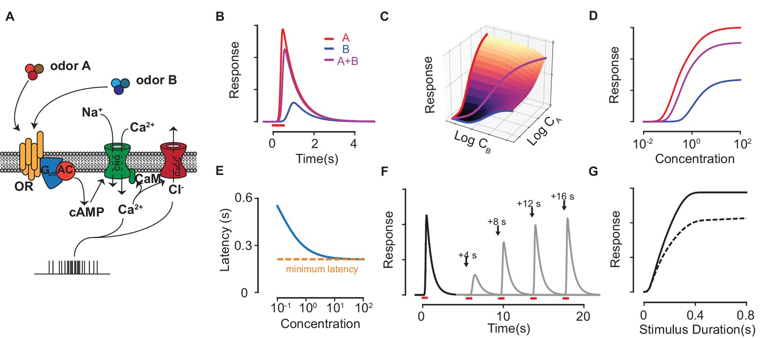
Response properties of an ORN in our biophysical model.

(A) Scheme of the modeled ORN signal transduction pathway. (B) The temporal responses of an ORN to odorants $A$ (red) and $B$ (blue) delivered separately and as a mixture (magenta). (C–D) The peak response of the mixture for different concentrations of $A$ and $B$ . The three colored curves in (C) are plotted separately in (D) on a single axis, whose scale corresponds to $C_{A}$ , $C_{B}$ and $C_{A} + C_{B}$ for $A$ , $B$ and the mixture $A + B$ , respectively. (E) The response latency vs odorant concentration. The red, dashed line shows the minimum possible latency due to the limiting receptor activation and cAMP production steps in the signal transduction, which varies between a few tens of milliseconds to a few hundred milliseconds depending on the particular odorant-receptor pair under consideration (Ghatpande and Reisert, 2011; Rospars et al., 2003). (F–G) The Ca $^{2 +}$ -based adaptation properties of the biophysical model. In (F) the first odorant pulse at $t = 0$ is followed by a second pulse at each of the four shown times in separate trials. Full response is recovered after a few tens of seconds. (G) The peak response of a pulse (solid) and a second pulse (dashed) delivered 10 s later against the pulse duration of both pulses.

https://doi.org/10.7554/eLife.34958.003

Figure 2

Download asset Open asset

Suppression due to masking.

(A) The dashed line shows the response predicted by our model with only the first odorant (delivered during the red time window), while the solid line shows the predicted response when a second pulse of a highly masking odorant is delivered shortly after during the green window (plotted as in (Kurahashi et al., 1994)). (B) Experimental data on the masking effect of various masking agents (circles) and fits to theory (lines). Blue: 2,4,6-trichloroanisole, red: 2,4,6-tribromoanisole, yellow: phenol, Magenta: 2,4,6-trichlorophenol, cyan: trichlorophenetole, black: L-cis diltiazem, green: geraniol. (C–D) Mixture response curves displaying synergy (C) and inhibition (D). The curves are plotted as in Figure 1D.

https://doi.org/10.7554/eLife.34958.004

Figure 3

Download asset Open asset

The encoding model.

(A) The response curves of a collection of 10 ORN types to an odorant. The vector $y$ of continuous levels of response at a particular concentration (red, dashed line) yields a binary vector $z$ of activation by imposing a threshold $τ$ (blue, dashed). (B) For a particular ORN type, the sensitivities of the five most sensitive odorants in a mixture relative to the sensitivity of the most sensitive odorant are shown. Blue, orange and green colors correspond to the number of components in the mixture, $n_{mix} =$ 10, 50 and 100 respectively. (C) The relative error due to the approximation in (4) for $κ_{mix}^{- 1}$ (red) and $η_{mix}$ (blue) as a function of $n_{mix}$ . Solid lines refer to an equiproportionate mixture. Conversely, dashed lines refer to the case where concentrations are drawn uniformly in log scale over six orders of magnitude. The comparison indicates that our approximations in the main text become even better when the concentrations are variable.

https://doi.org/10.7554/eLife.34958.005

Figure 4 with 1 supplement

Download asset Open asset

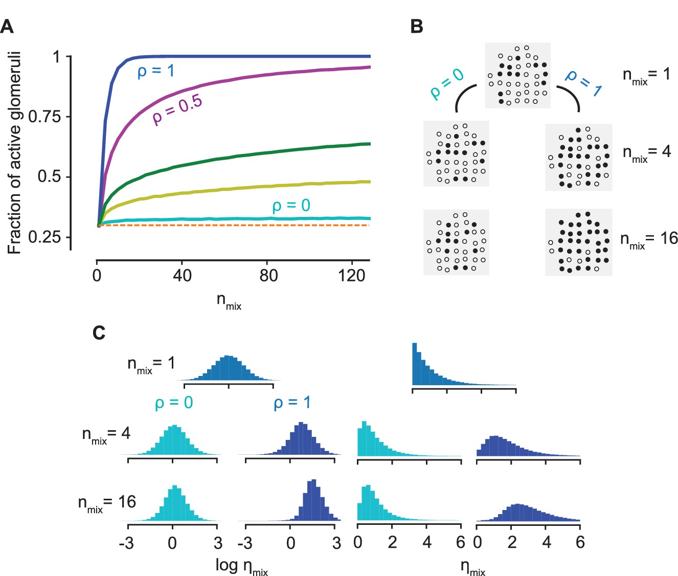
Normalization due to antagonism.

(A) The fraction of active glomeruli as the number of odorants in the mixture, $n_{mix}$ , increases, each of which individually activates 30% of the glomeruli ( $ρ = 0, 0.1, 0.2, 0.5, 1$ from the bottom to the top curves). (B) The glomerular pattern of activation for $ρ = 0$ and $ρ = 1$ for three values of $n_{mix}$ , shown to contrast the sparsity of their glomerular responses. (C) The distribution of the activation efficacy $η_{mix}$ over different ORN types for $ρ = 0$ (cyan) and $ρ = 1$ (blue) as $n_{mix}$ increases, where $η$ for each component is drawn from a log-normal (left) or an exponential distribution (right). The distribution is largely invariant w.r.t $n_{mix}$ for $ρ = 0$ , whereas it gets increasingly biased toward higher values for $ρ = 1$ . Normalization is independent of the sparsity of activation (see Figure 4—figure supplement 1).

https://doi.org/10.7554/eLife.34958.006

Figure 4—figure supplement 1

Download asset Open asset

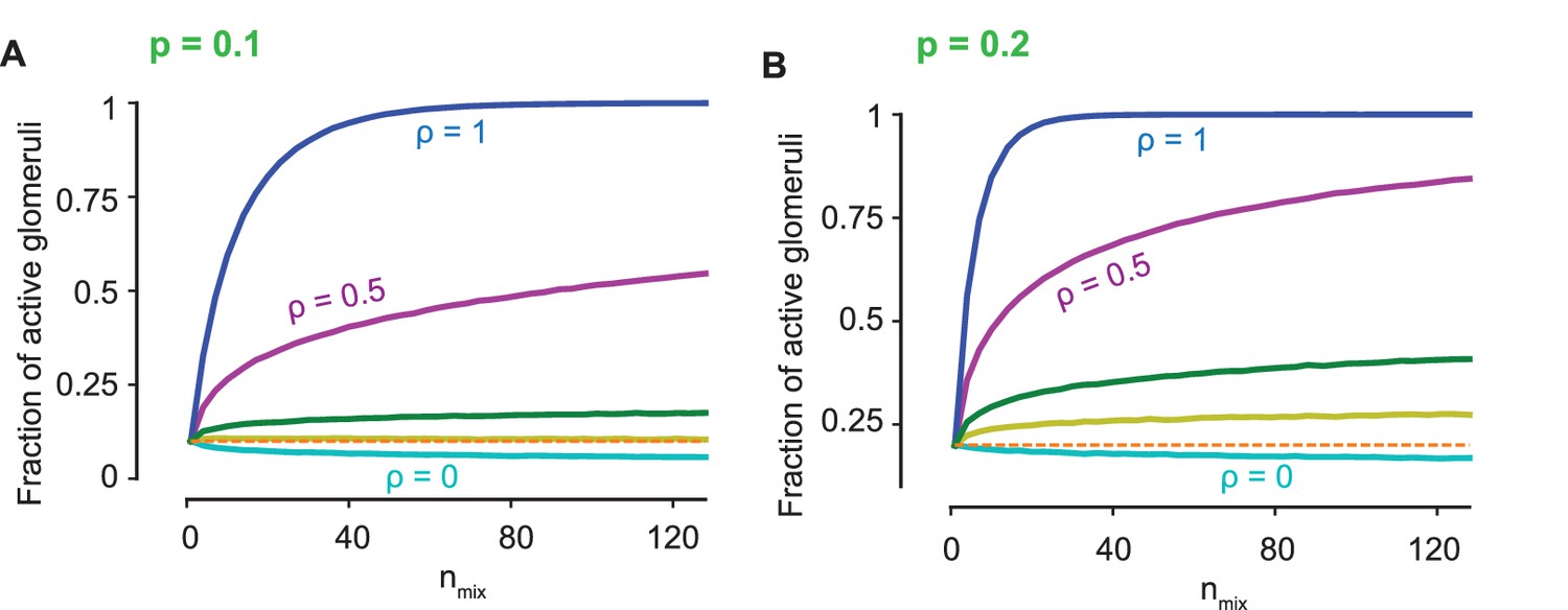
Normalization is independent of the sparsity of activation: The fraction of active glomeruli against the number of odors in the mixture, $n_{mix}$ , is shown as in Figure 4A for sparsity $p$ = 0.1 and $p$ = 0.2.
https://doi.org/10.7554/eLife.34958.007

Figure 5 with 1 supplement

Download asset Open asset

The positive effects of antagonism on odor discrimination and component separation.

(A–B) Figure-ground segregation: (A) The mutual information between the presence of a target odorant and the glomerular activation vector $z$ for the antagonistic factor (13) $ρ = 0$ (cyan), 0.5 (magenta), 1 (blue) with varying number of background odorants in the mixture. (B) The optimal value $ρ^{*}$ of the antagonistic factor $ρ$ that maximizes mutual information when the number of background odorants vary from trial to trial for different sparsity levels $p$ i.e. the fraction of glomeruli that are activated. The yellow region marks experimentally observed levels of sparsity. The inset shows how the mutual information varies for three values of the sparsity. (C–D) Component separation: ROC curves (the hit rate vs the number of false positives (FPs)) are shown for three values of $ρ$ (color scheme as in panel A) and two relevant values of $p$ . Inset: Same curves in semi-log scale. The positive effect of antagonism is retained in the case where there is significant internal noise (see Figure 5—figure supplement 1).

https://doi.org/10.7554/eLife.34958.008

Figure 5—figure supplement 1

Download asset Open asset

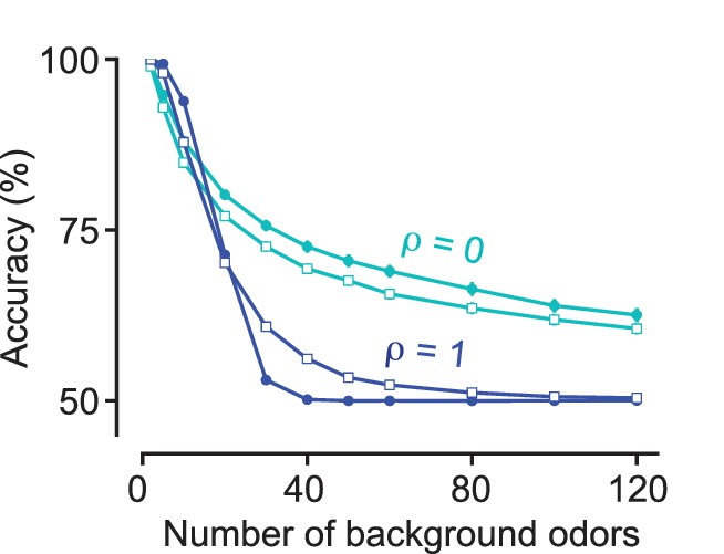
Performance is largely independent of internal noise: The accuracy of a linear classifier in detecting a target odorant is plotted against the number of background odorants for $ρ = 0$ (cyan) and $ρ = 1$ (blue), where an effective internal noise of magnitude $ϵ$ is added (see Materials and methods).

The curves with solid circles correspond to $ϵ = 0$ and the open squares correspond to $ϵ$ = 0.4.

https://doi.org/10.7554/eLife.34958.009

Figure 6 with 1 supplement

Download asset Open asset

Antagonism and psychophysics.

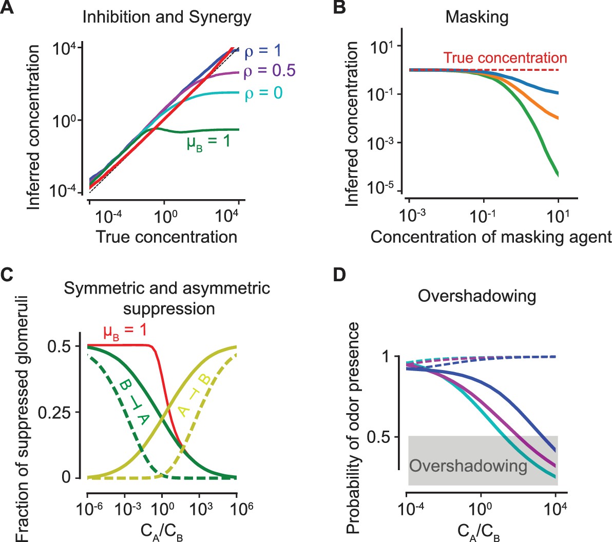
(A) Inhibition and synergy: The inferred vs the true concentration for a single odorant $A$ (solid, red line) or with an additional odorant $B$ . Blue, magenta, cyan: $ρ = 1, 0.5, 0$ , as defined in (5). Green line: the inferred concentration when $B$ has a high masking coefficient $μ_{B}$ , as defined in (18) and (20). In all panels, the sparsity of glomerular activation is $p = 0.5$ . (B) Masking: The inferred concentration of $A$ for increasing concentrations of a masking agent $B$ (blue, orange, green: $μ_{B} = 0.4, 0.7, 1$ ). (C) Symmetric and asymmetric suppression: The fraction of suppressed glomeruli of $A$ ( $B$ ) is plotted in green (yellow) against the ratio of concentrations of $A$ and $B$ . Solid/dashed lines: $ρ = 0, 1$ . The red line shows the fraction of suppressed glomeruli when $B$ also has a propensity for masking. (D) Overshadowing: The probability of presence of $B$ as computed by the logistic regressor against the ratio of $A$ and $B$ concentrations. The dashed lines show the probability of presence of $A$ . Color code is as in panel (A). The above results are independent of the sparsity of activation (see Figure 6—figure supplement 1).

https://doi.org/10.7554/eLife.34958.010

Figure 6—figure supplement 1

Download asset Open asset

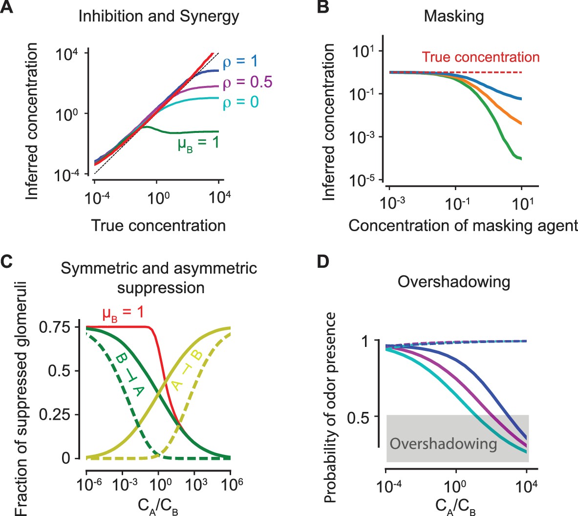
Predicted psychophysical effects of antagonism are independent of the sparsity of activation: The results as shown in Figure 6 for sparsity $p = 0.25$ to show that our conclusions are independent of the sparsity level.
https://doi.org/10.7554/eLife.34958.011

Additional files

Transparent reporting form: https://doi.org/10.7554/eLife.34958.012
Download elife-34958-transrepform-v1.docx

Download links

A two-part list of links to download the article, or parts of the article, in various formats.

Downloads (link to download the article as PDF)

Open citations (links to open the citations from this article in various online reference manager services)

Mendeley

Cite this article (links to download the citations from this article in formats compatible with various reference manager tools)

Gautam Reddy
Joseph D Zak
Massimo Vergassola
Venkatesh N Murthy

(2018)

Antagonism in olfactory receptor neurons and its implications for the perception of odor mixtures

eLife 7:e34958.

https://doi.org/10.7554/eLife.34958

Sign up for email alerts

Privacy notice