Genetics of trans-regulatory variation in gene expression
- University of Minnesota, United States
- University of California, Los Angeles, United States
- Howard Hughes Medical Institute, United States
Figures
Figure 1 with 2 supplements
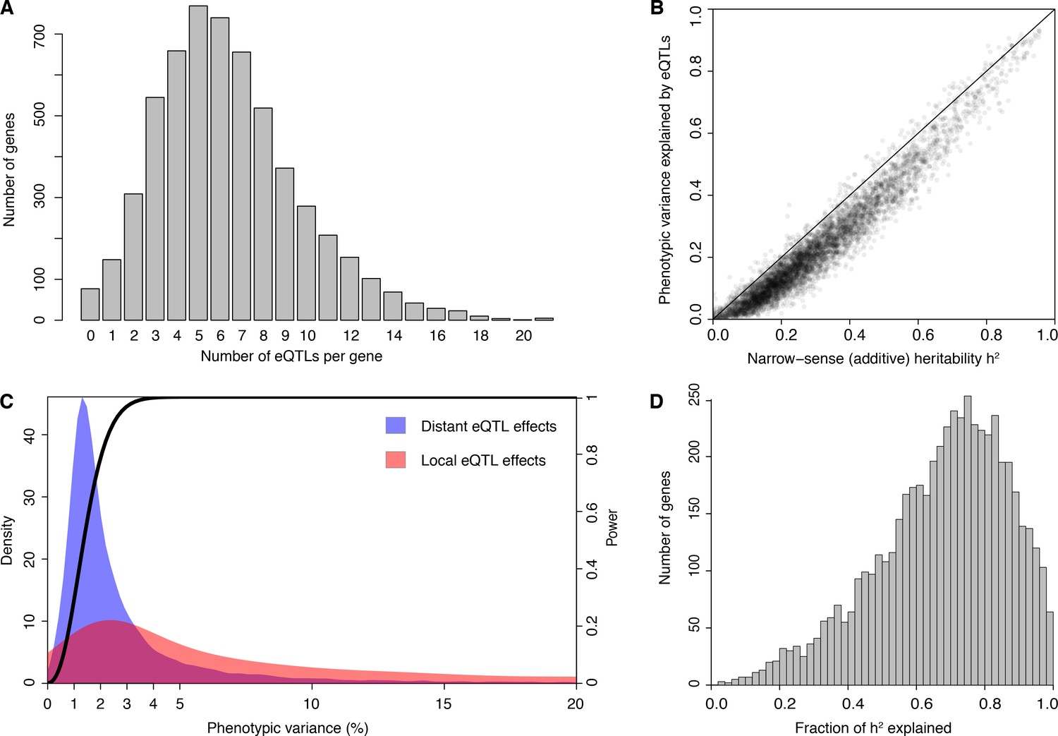
eQTL detection and transcriptome heritability.
(A) Histogram showing the number of eQTLs per gene. (B) Most additive heritability for transcript abundance variation is explained by detected eQTLs. The total variance explained by detected eQTLs for each transcript (y-axis) is plotted against the additive heritability (h2). The diagonal line represents a scenario under which the variance explained by eQTLs exactly matches the heritability. (C) Power to detect eQTLs as a function of effect size, and distributions of observed local and distant eQTL effects. The black curve corresponds to the statistical power (right y-axis) for eQTL detection at a genome-wide significance threshold. Colored areas show the density of individual significant eQTLs (left y-axis) that explain a given fraction of phenotypic variance (x-axis) for distant (blue) and local (red) eQTLs. Note that the x-axis is truncated at 20% variance explained to aid visualization of smaller effects, and omits a long tail of few eQTLs with large effects. (D) Histogram showing the fraction of h2 explained by the sum of the eQTLs for each gene.
Figure 1—figure supplement 1
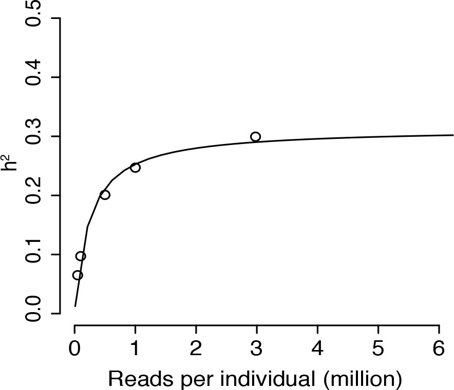
Mean additive heritability across all transcripts as a function of downsampling the total number of reads per sample.
The downsampled number of reads per sample (x-axis) is plotted against the mean additive heritability across all genes (y-axis). The black line is a non-linear least squares fit.
Figure 1—figure supplement 2

Heritability (h2) compared to other measures.
In all panels, heritability for each gene is plotted on the y-axis and compared to: (A) The average log2(TPM) for a gene across the segregants. (B) The number of detected eQTLs per gene. (C) The fraction of phenotypic variance explained by the largest effect eQTL per gene. The diagonal line represents the case of all heritability mapping to the strongest eQTL. (D) The fraction of additive heritability explained by the largest effect eQTL per gene. The vertical line represents the case of all additive heritability being explained by the strongest eQTL.
Figure 2 with 2 supplements
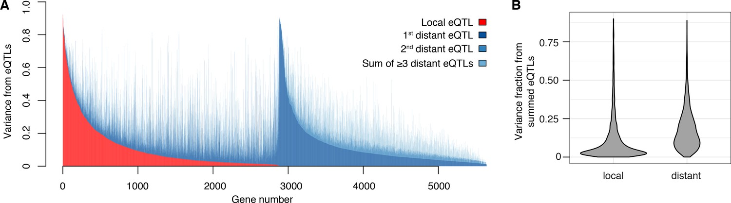
Contribution of local and distant eQTLs to expression variance.
(A) A stacked barplot showing for each gene with at least one eQTL the amount of phenotypic variance from local and distant eQTLs. Genes are sorted first by the amount of variance from the local eQTL, followed by the amount of variance from the strongest distant eQTL. (B) Violin plots of the distributions of fractions of phenotypic variance explained by summed local and distant eQTLs, respectively. This panel was generated using genes with at least one local and one distant eQTL.
Figure 2—figure supplement 1
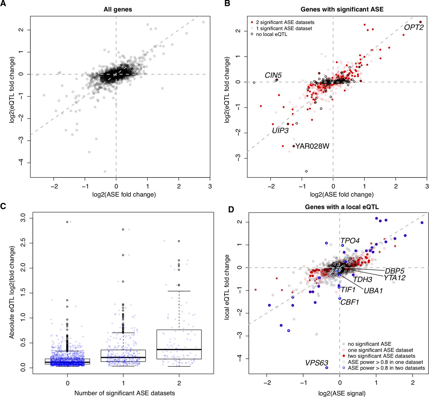
Allele-specific expression (ASE) compared to local eQTL effects.
(A) For each gene present in the ASE datasets, we show the magnitude of ASE in the diploid BY/RM hybrid (x-axis) vs. the magnitude of the local eQTL in the current data (y-axis). Positive values indicate higher expression in RM compared to BY. The vertical and horizontal lines indicate ASE and local eQTL effects of zero, respectively. The diagonal line represents identical ASE and local eQTL effects. Local eQTL effects are computed for all genes, irrespective of whether the local eQTLs were significant. (B) As in (A), but showing only genes with significant ASE in at least one ASE dataset. Black circles: genes without a significant local eQTL. We show names of genes that have ASE in both datasets but do not have a significant local eQTL. (C) Boxplots showing absolute local eQTL effects for genes with no, one, or two significant ASE datasets. (D) as in (A), but only for genes with a significant local eQTL. Blue circles: genes with high statistical power to detect ASE. We show the names of genes with a local eQTL and high ASE power but no significant ASE, and names of genes with significant ASE and a local eQTL with opposite direction of effect (TDH3, YTA12, DBP5).
Figure 2—figure supplement 2

Power to detect allele-specific expression.
The figure shows the results from a simulation study that varied the strength of true ASE (x-axis) and the depth of sequencing coverage, expressed as the number of reads covering the two alleles of the gene. Different depths of coverage are shown as colored lines. The blue line indicates the median coverage per gene observed in (Albert et al., 2014a), and the grey lines indicate the 10th and 90th coverage quantile in the same reference. The green area indicates the fold-changes observed for local eQTLs to show the ASE magnitudes that may be expected in real data. On the y-axes, the panels show: Left: Power to detect ASE at nominal significance of p≤0.05, Middle: Power to detect ASE with Bonferroni correction across the number of expressed genes, Right: the fraction of simulated ASE datasets in which the observed direction of ASE matched the true direction, irrespective of statistical significance.
Figure 3
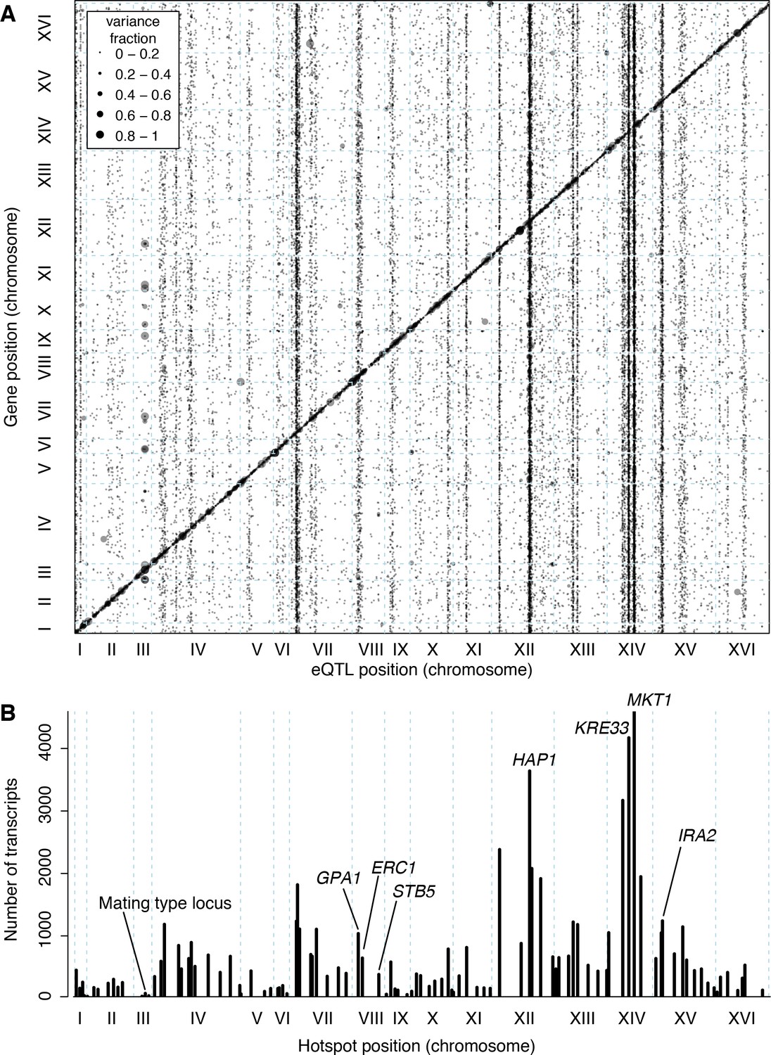
Locations of eQTLs in the genome.
(A) Map of local and distant eQTLs. The genomic locations of eQTL peaks (x-axis) are plotted against the genomic locations of the genes whose expression they influence (y-axis). The strong diagonal band corresponds to local eQTLs. The many vertical bands correspond to eQTL hotspots. Point size is scaled as a function of eQTL effect size, measured in fraction of phenotypic variance explained. (B) The number of gene expression traits linking to each of 102 identified eQTL hotspots (Methods) are shown as vertical bars. Text labels identify genes in hotspots referred to in the text.
Figure 4 with 4 supplements
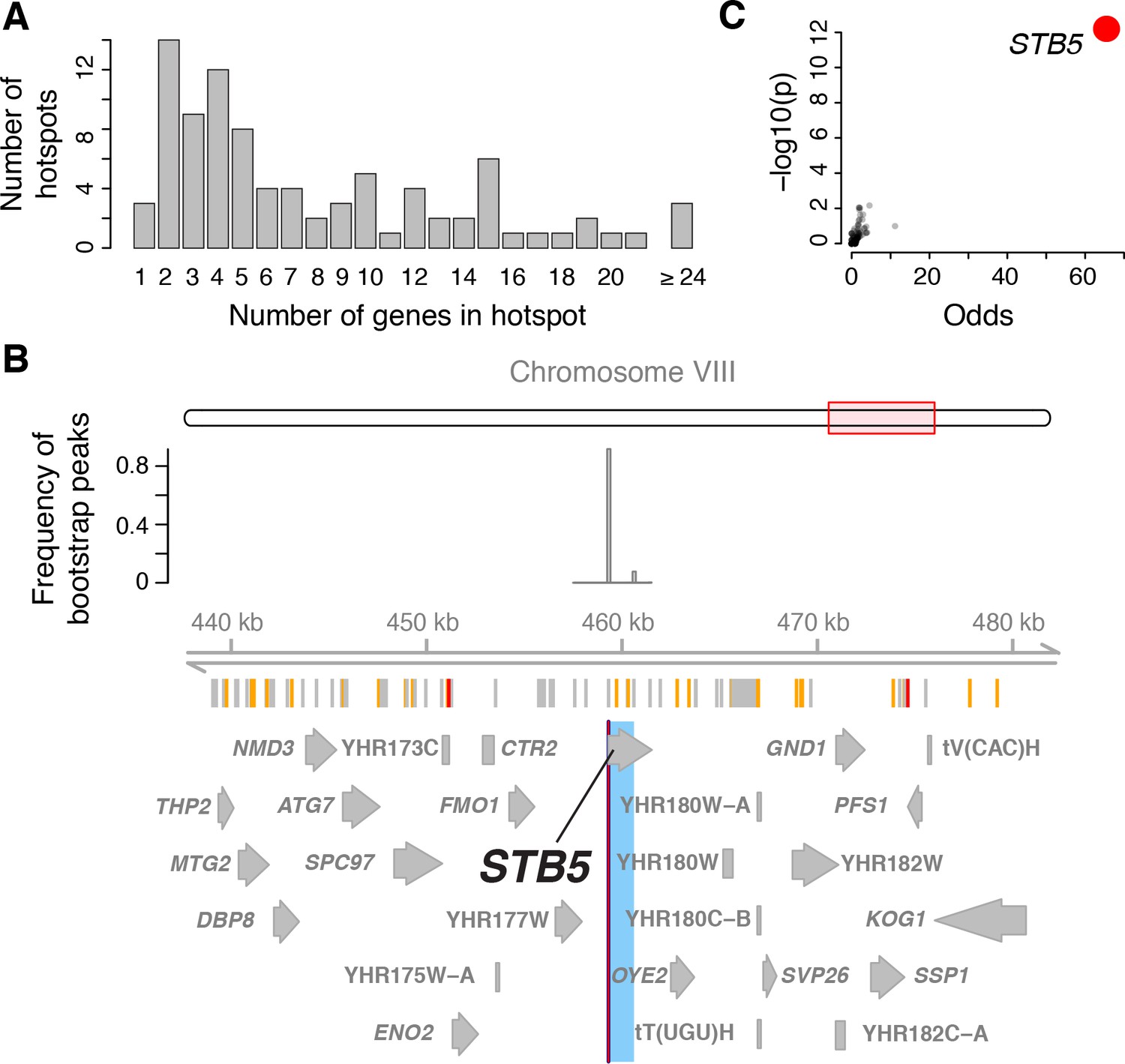
Genes located in hotspot regions.
(A) Histogram showing the number of genes located in the hotspot regions. (B) A hotspot on chromosome VIII maps to the gene STB5. From top to bottom: the general region on the chromosome, the empirical frequency distribution of hotspot peak locations from 1000 bootstrap samples (Materials and methods), locations of BY/RM sequence variants (red: variants with ‘high’ impact such as premature stop codons (McLaren et al., 2016); orange: ‘moderate’ impact such as nonsynonymous variants; grey: ‘low’ impact such as synonymous or intergenic variants), and gene locations. The light blue area shows the 95% confidence interval of the hotspot location as determined from the bootstraps. The red line shows the position of the most frequent bootstrap marker. (C) Genes for which the BY allele at the STB5 hotspot is linked to lower expression are enriched for STB5 transcription factor (TF) binding sites in their promoter regions. The figure shows enrichment results for all annotated TFs (grey dots), with the strength of enrichment (odds ratio) on the x-axis vs. significance of the enrichment on the y-axis. The STB5 result is highlighted in red.
Figure 4—figure supplement 1
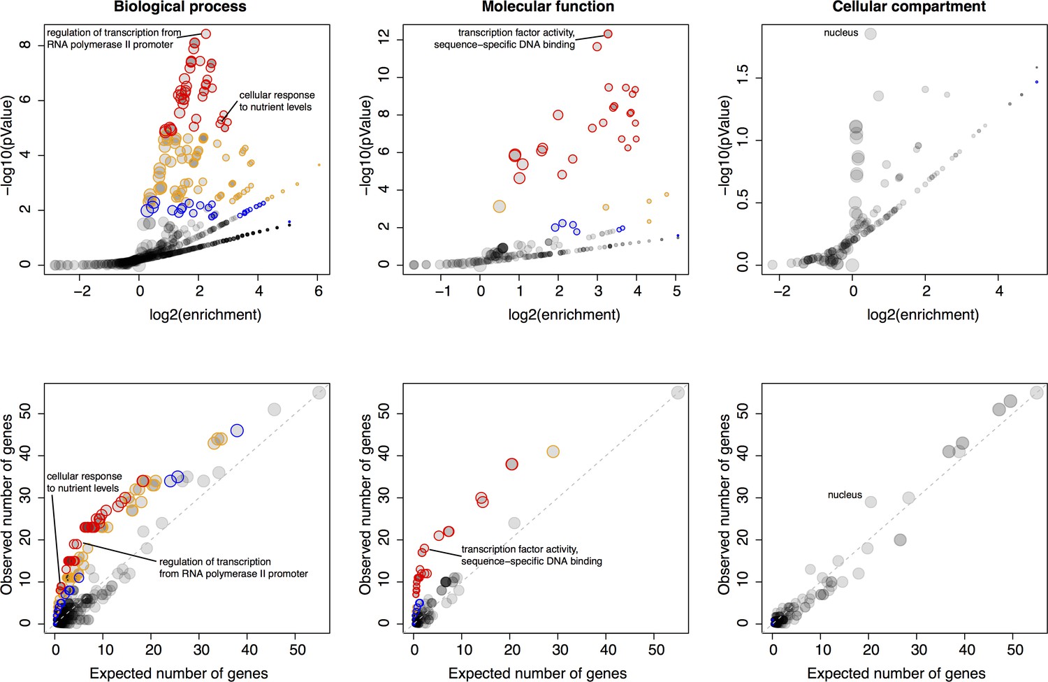
Gene ontology (GO) enrichments of genes located in hotspots.
For each major GO category of ‘Biological Process’, ‘Molecular Function’, and ‘Cellular Compartment’, the figure shows two panels. The most significant GO term as well as GO terms discussed in the main text are indicated. Top panels: Relationship between strength (x-axis) and significance (y-axis) of the GO enrichment. Each GO term is plotted as a dot, with size scaled as a function of the number of terms in the GO group. Note how the relationship between enrichment strength and significance depends on GO category size. Different levels of significance are indicated by colored circles. With decreasing stringency, these colors indicate: Red: p<0.05 after Bonferroni correction for the number of GO terms tested; Orange: permutation-based p<0.005, corresponding to an FDR of 5% (Materials and methods), Blue: GO term specific permutation-based p<0.01. Bottom panels: The number of genes in each GO term expected to be significant based on GO category size (x-axis) vs. the number of genes in each GO term observed to be significant. Color codes are as in the top panels. The diagonal line indicates observations that match the expectation.
Figure 4—figure supplement 2
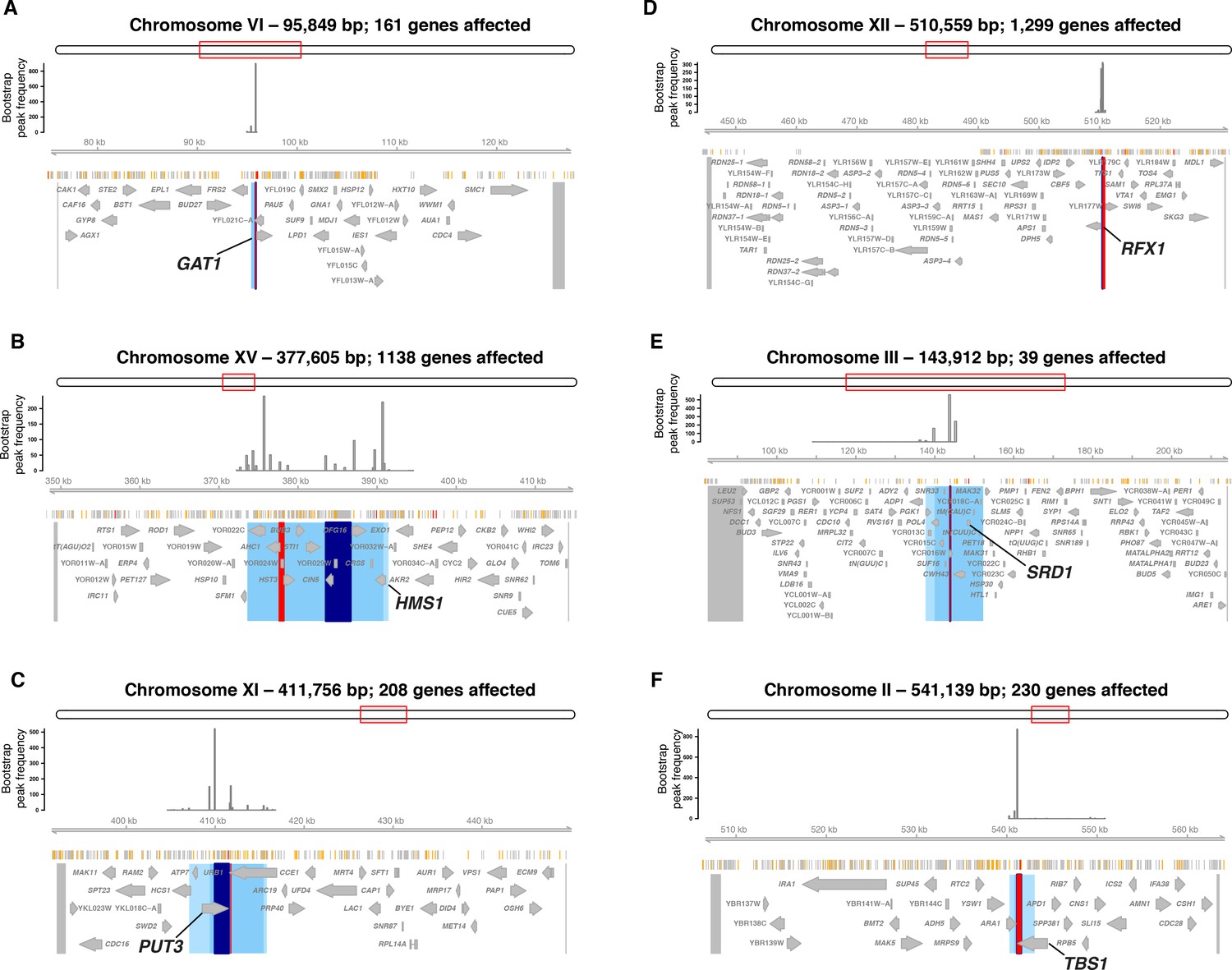
Hotspots at six transcription factor genes with damaging mutations.
Each panel shows the region surrounding one hotspot containing (A) GAT1, (B) HMS1, (C) PUT3, (D) RFX1, (E) SRD1, and F) TBS1. Panel elements are as in Figure 4. Blue area shows the 90% confidence interval of hotspot location, and lighter blue areas shows the 95% confidence interval. The entire region tested in the bootstrap analysis is delimited by two markers shown as grey lines at the outer edges of the plots. These markers and the peak markers are padded to span all variants that are in perfect linkage disequilibrium with the given marker.
Figure 4—figure supplement 3
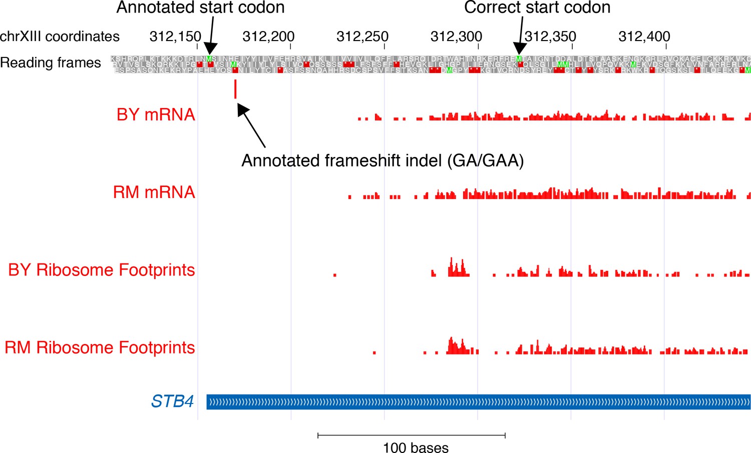
mRNA and translation at STB4.
The figure shows the position of the first base in aligned reads from mRNA sequence and ribosome profile data (Albert et al., 2014a) in BY and RM. The annotated frameshift is located in a region without any mRNA or ribosome footprint reads. The annotated (presumably incorrect) and the likely correct start codon of STB4 are indicated.
Figure 4—figure supplement 4
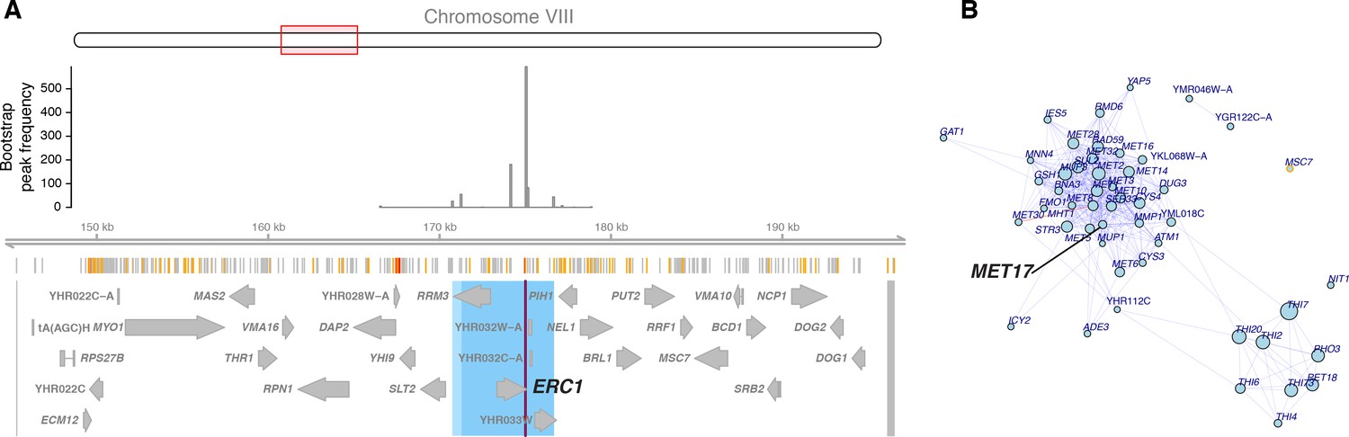
The ERC1 hotspot.
(A) The region surrounding the ERC1 hotspot. Legend as in Figure 4B. The entire region tested in the bootstrap analysis is delimited by two markers shown as grey lines at the outer edges of the plots. These markers and the peak markers are padded to span all variants that are in perfect linkage disequilibrium with the given marker. (B) A visual representation of the top 50 genes affected by the hotspot. Each gene is shown as a dot, with size scaled as a function of the size of the effect of the hotspot on the gene. We show genes with lower expression linked to the BY allele. Genes with a local eQTL anywhere in the region tested in the bootstrap analysis are indicated by orange circles. Edges between genes indicate co-expression in a gene regulatory network (Zhang and Kim, 2014). Blue edges: positive co-expression, red edges: negative co-expression. Note the group of genes with methionine-related functions, including MET17.
Figure 5

Relationship of local eQTLs and distant eQTL hotspots.
(A) The fraction of hotspots that contain a genome-wide significant local eQTL. The black histogram shows the distribution observed in 1000 random, size-matched regions of the genome. Because of the high number of local eQTLs, most hotspots are expected to contain a local eQTL even by chance. The observed fraction (red line) still exceeds this random expectation. (B) Distribution of trans eQTLs at local eQTLs outside of hotspot regions. The genome was divided into non-overlapping bins centered on local eQTLs that did not overlap a hotspot. We counted the number of trans-eQTL peaks in each bin. The figure shows the frequency of bins with a given number of trans-eQTLs. The distribution observed in real data is shown by red lines, and distributions obtained in 1000 randomizations of trans-eQTL positions is show by clouds of black circles. The inset shows the observed less the expected frequency for each bin. Error bars indicate the 95% range from the randomizations.
Figure 6
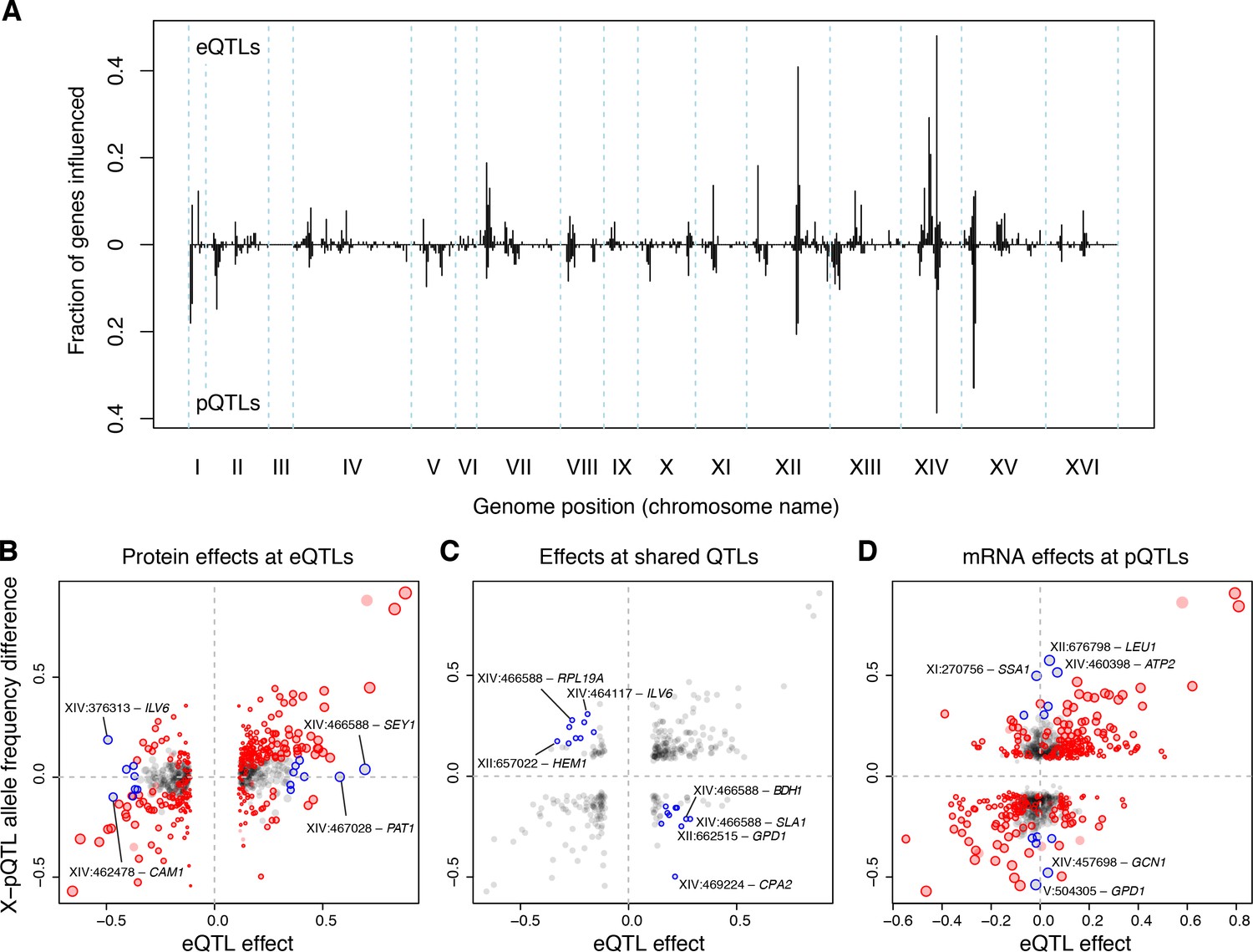
eQTLs and pQTLs.
(A) Distant eQTL and pQTL hotspots. The figure shows the fraction of 154 genes (Albert et al., 2014b) that have an eQTL or pQTL in a given bin along the genome. eQTLs from the current dataset are shown in the upper half of the figure, and pQTLs from (Albert et al., 2014b) are shown in the bottom half with an inverted scale. Chromosome III is omitted from the figure because no pQTLs can be detected on this chromosome due to the experimental design of (Albert et al., 2014b). (B–D) Comparison of individual distant eQTLs and pQTLs. Each panel shows the effect size of linkage of mRNA levels for a given gene to a given genomic position (x-axis; correlation coefficient between mRNA level and marker genotype) compared to the effect size of linkage of protein levels for the same gene to the same genomic position (y-axis; difference in frequency of the BY allele between segregant pools with high and low expression of the protein [Albert et al., 2014b]). Positive values indicate higher expression in RM compared to BY. Only distant QTLs located on different chromosomes than their target gene are shown. (B) All distant eQTLs, irrespective of significance in pQTL data. Dot size scales as a function of eQTL effect size. Red circles: eQTLs that overlap a significant pQTL. Blue circles: strong eQTLs that do not overlap a pQTL (Supplementary file 8); extreme cases are indicated by QTL location and the name of the affected gene. (C) Overlapping significant eQTLs and significant pQTLs. Blue circles: overlapping QTLs with different direction of effect (Supplementary file 9); extreme cases are indicated. (D) All distant pQTLs, irrespective of significance in eQTL data. Dot size scales as a function of pQTL effect size. Red circles: pQTLs that overlap a significant eQTL. Blue circles: strong pQTLs that do not overlap an eQTL (Supplementary file 10); extreme cases are indicated.
Figure 7 with 3 supplements
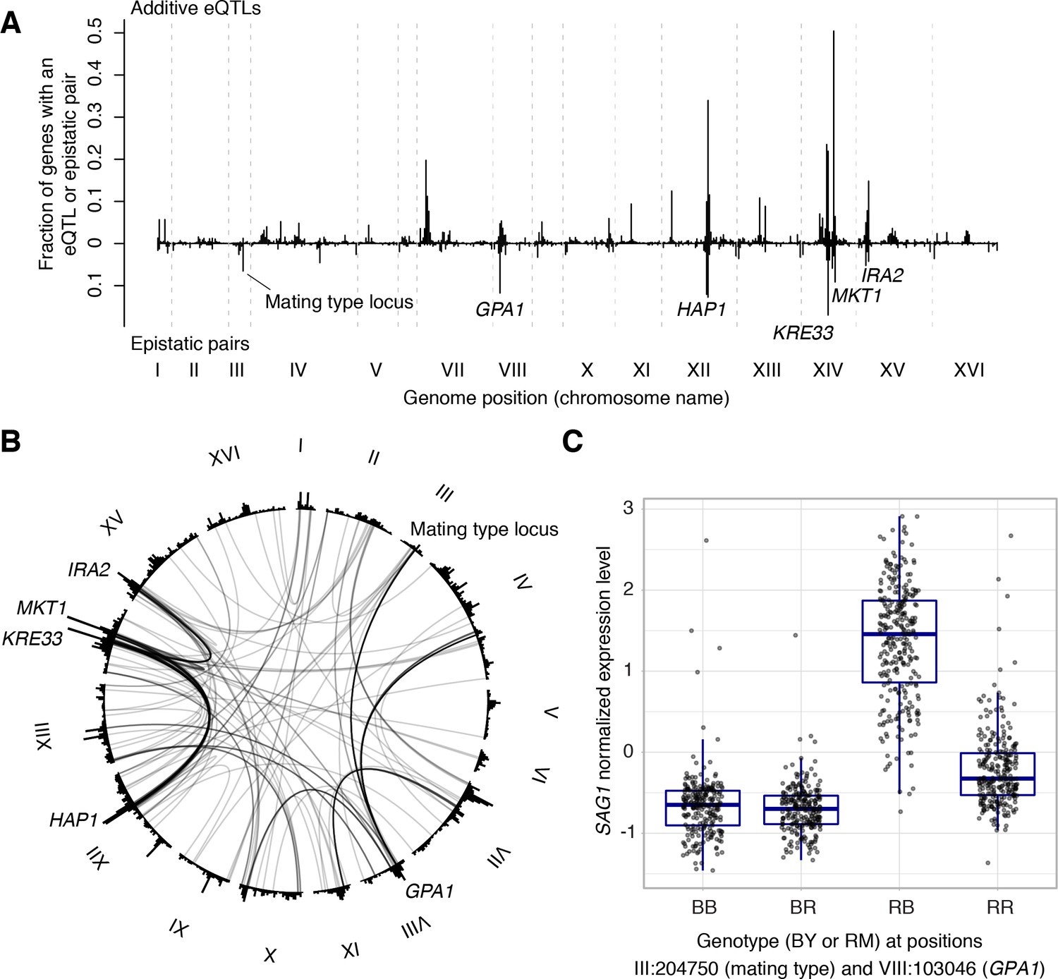
Non-additive interactions between eQTLs.
(A) Locations of markers of epistatic pairs (pointing downward) compared to those of additive eQTLs (pointing upward). Epistatic hotspots discussed in the text are highlighted. (B) Interactions between two trans loci. The plot shows the genome broken up into chromosomes (indicated as roman numerals), with arches connecting two interacting loci. Arches are shaded such that multiple overlapping interactions appear darker. Epistatic hotspots are indicated as in panel A. The outer histogram shows the density of additive eQTLs. (C) Expression levels of SAG1 as a function of genotypes at the mating type locus and GPA1.
Figure 7—figure supplement 1
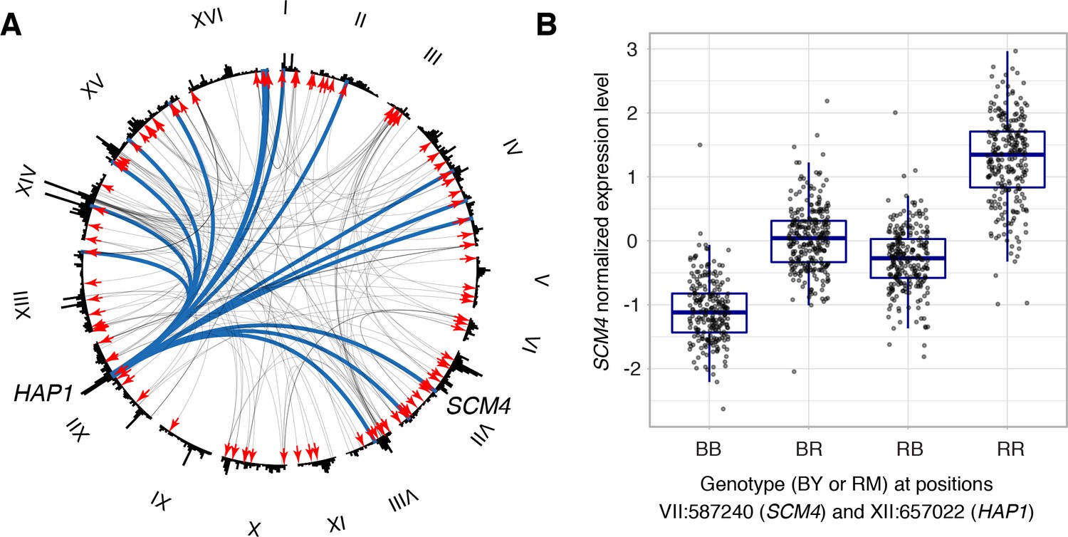
Cis by trans interactions.
(A) Interactions between trans and local loci. The plot shows the genome broken up into chromosomes (indicated as roman numerals), with arches connecting two interacting loci. Arches are shaded such that multiple overlapping interactions appear darker. Red arrows denote the local eQTLs. Blue lines indicate the interactions involving the HAP1 locus. The example shown in panel B is indicated. The outer histogram shows the density of additive eQTLs. (B) Expression levels of SCM4 as a function of genotypes at HAP1 and the SCM4 locus.
Figure 7—figure supplement 2
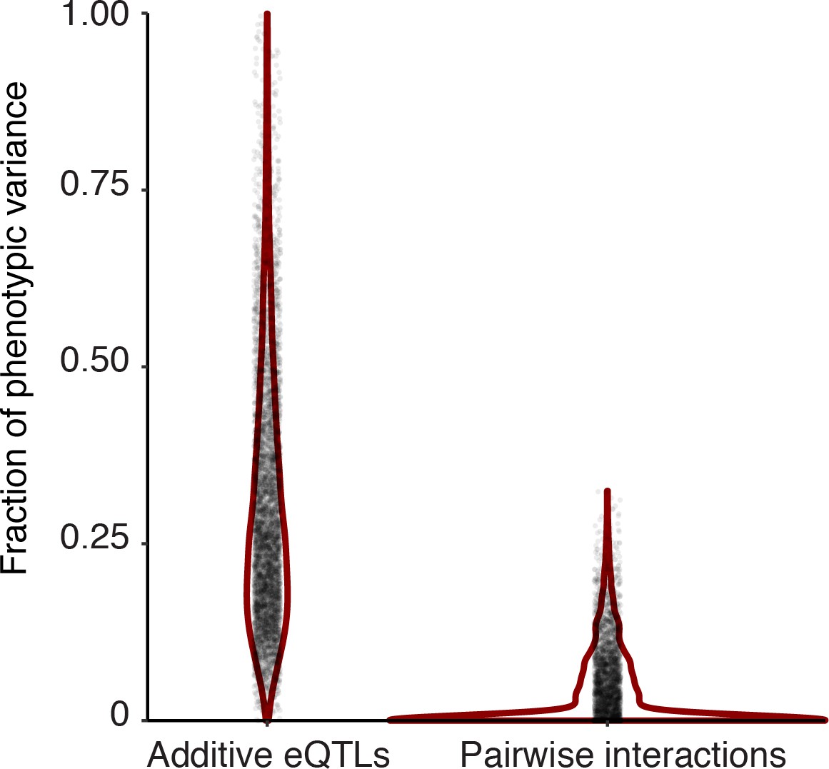
Distribution of the fraction of phenotypic variance (y-axis) explained by genetic variation as captured by genome-wide relatedness in an additive (left), and interactive (right) model.
https://doi.org/10.7554/eLife.35471.019
Figure 7—figure supplement 3
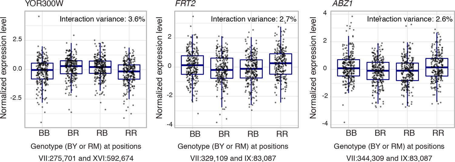
Epistatic interactions without additive effects.
Shown are expression levels of three genes without any additive signal at either of the two interacting markers.
Additional files
-
Source data 1
Expression values.
This xlsx file contains expression levels in units of log2(TPM) for all genes and segregants.
- https://doi.org/10.7554/eLife.35471.021
-
Source data 2
Covariates.
This xlsx file contains information on experimental batch and growth covariates for all segregants.
- https://doi.org/10.7554/eLife.35471.022
-
Source data 3
Genotypes.
This xlsx file contains genotypes at 42,052 markers for all segregants. BY (i.e. reference) alleles are denoted by ‘−1’. RM alleles are denoted by ‘1’.
- https://doi.org/10.7554/eLife.35471.023
-
Source data 4
Detected eQTLs.
This xlsx file contains all detected eQTLs.
- https://doi.org/10.7554/eLife.35471.024
-
Source data 5
Heritability estimates.
This xlsx file contains additive and pairwise interactive genetic variance estimates for all genes.
- https://doi.org/10.7554/eLife.35471.025
-
Source data 6
Gene characteristics and annotations.
This xlsx file contains gene features used for comparisons with heritability.
- https://doi.org/10.7554/eLife.35471.026
-
Source data 7
Data for allele-specific expression comparisons.
This xlsx file contains processed data used to compare ASE and local eQTLs.
- https://doi.org/10.7554/eLife.35471.027
-
Source data 8
Overview of eQTL hotspots.
This xlsx file presents information on the detected hotspots such as position, number of genes affected, genes located in the region, GO and transcription factor binding site enrichments of the affected genes. The file has a legend in a separate work sheet.
- https://doi.org/10.7554/eLife.35471.028
-
Source data 9
Hotspot effect matrix.
This xlsx file contains estimated effects of all hotspots on all genes.
- https://doi.org/10.7554/eLife.35471.029
-
Source data 10
GO enrichment results for genes affected by each hotspot.
This txt file contains GO enrichment results for the 102 hotspots in one file. Columns indicate hotspot identity, GO subcategory (‘biological process’, ‘molecular function’, or ‘cellular compartment’), and the group of genes tested for enrichment (‘RM’=up to 100 genes with the strongest hotspot effects with higher expression linked to the RM allele, ‘BY’=as for ‘RM’, but higher expression linked to the BY allele).
- https://doi.org/10.7554/eLife.35471.030
-
Source data 11
Enrichments for transcription factor binding sites at genes affected by each hotspot.
This txt file contains enrichment results for the 102 hotspots in one file. Columns indicate hotspot identity, and the group of genes tested for enrichment (‘RM’=up to 100 genes with the strongest hotspot effects with higher expression linked to the RM allele, ‘BY’=as for ‘RM’, but higher expression linked to the BY allele).
- https://doi.org/10.7554/eLife.35471.031
-
Source data 12
GO enrichment results for genes located in hotspots.
This xlsx file contains the results of a GO enrichment analysis of genes physically located in hotspot regions.
- https://doi.org/10.7554/eLife.35471.032
-
Source data 13
Comparison with pQTLs.
This xlsx file contains processed data used for the comparisons of eQTLs and pQTLs.
- https://doi.org/10.7554/eLife.35471.033
-
Source data 14
Detected interactions between eQTL pairs.
This xlsx file contains all detected pairs of eQTLs with non-additive genetic interactions. There are separate sheets for the genome-wide scan, the scan between additive eQTLs and the genome, and the scan between additive eQTLs. There is also a legend in a separate sheet.
- https://doi.org/10.7554/eLife.35471.034
-
Supplementary file 1
Multiple regression of heritability on various gene features.
Sums of squares, degrees of freedom and F-values were computed using Type II analysis of variance as implemented in the R car package. (1) log2(TPM).
- https://doi.org/10.7554/eLife.35471.035
-
Supplementary file 2
Genes with strong (more than 2-fold) and significant ASE in both datasets but no local eQTL.
(1) Shown is the less significant p-value from the two ASE datasets. (2) The LOD score at the gene position itself irrespective of whether this eQTL is significant. (3) Positive values indicate higher expression in RM compared to BY. (4) These genes have strong eQTLs close to the gene, but with a confidence interval that just excludes the gene. The may be influenced by cis acting local eQTLs where the causal variant is located further away from the gene than captured by our definition of upstream regulatory regions as 1000 base pairs upstream of the start codon.
- https://doi.org/10.7554/eLife.35471.036
-
Supplementary file 3
Genes with a local eQTL but no ASE in spite of ≥80% power to detect ASE.
(1) Positive values indicate higher expression in RM compared to BY. (2) Shown is the more significant p-value from the two ASE datasets. (3) The nominally significant p-values in this column do not pass Bonferroni cutoff for significance. Therefore, ASE at these genes was not identified as significant.
- https://doi.org/10.7554/eLife.35471.037
-
Supplementary file 4
Genes with a local eQTL and significant ASE, and discordant direction of effect.
(1) Positive values indicate higher expression in RM compared to BY. (2) Shown is the less significant p-value from the two ASE datasets. (3) The table shows only genes where both ASE datasets agreed in the direction of effect. Shown is the average effect.
- https://doi.org/10.7554/eLife.35471.038
-
Supplementary file 5
Hotspot region plots.
This pdf file contains one page per hotspot region, showing the position, bootstrap distribution, variant and gene content for each hotspot. See legend of Figure 4 and Figure 4—figure supplement 4 for further details.
- https://doi.org/10.7554/eLife.35471.039
-
Supplementary file 6
Plots of genes affected by hotspots.
This pdf file contains one page per hotspot region. Each page shows three gene co-expression networks. Each network displays connections among genes with the strongest linkages to the hotspot. The left plots show genes with higher expression in the presence of the RM allele. The middle plot shows genes with higher expression in the presence of the BY allele. The left and middle panels each show up to 50 genes with the strongest linkages to the hotspot in the given direction. If fewer than 50 genes were affected by the hotspot in the given direction, all genes affected in this direction are plotted, and their number indicated in the panel title. The right panel shows the joint network formed by the genes in the left and middle panel, with colors indicating up- or down-regulation by the hotspot. Genes with local eQTL located in the 95% confidence interval for hotspot location are indicated by red circles. Genes local eQTL located anywhere in the region tested by bootstraps are indicated by orange circles. See legend of Figure 4—figure supplement 4 for further details.
- https://doi.org/10.7554/eLife.35471.040
-
Supplementary file 7
Multiple logistic regression of genes located in hotspots on various gene features.
Likelihood ratios, degrees of freedom and p-values were computed using Type II analysis of variance as implemented in the R car package. (1) log2(TPM).
- https://doi.org/10.7554/eLife.35471.041
-
Supplementary file 8
Strong eQTLs without pQTL.
(1) Positive values indicate higher expression in RM compared to BY.
- https://doi.org/10.7554/eLife.35471.042
-
Supplementary file 9
Strong mRNA and protein QTLs with opposite effect.
(1) Positive values indicate higher expression in RM compared to BY.
- https://doi.org/10.7554/eLife.35471.043
-
Supplementary file 10
Strong pQTLs without eQTL.
(1) Positive values indicate higher expression in RM compared to BY.
- https://doi.org/10.7554/eLife.35471.044
-
Transparent reporting form
- https://doi.org/10.7554/eLife.35471.045
Download links
A two-part list of links to download the article, or parts of the article, in various formats.
Downloads (link to download the article as PDF)
Open citations (links to open the citations from this article in various online reference manager services)
Cite this article (links to download the citations from this article in formats compatible with various reference manager tools)
Genetics of trans-regulatory variation in gene expression
eLife 7:e35471.
https://doi.org/10.7554/eLife.35471


