Coordinated neuronal ensembles in primary auditory cortical columns
- University of California, San Francisco, United States
- University of California, United States
Figures
Figure 1
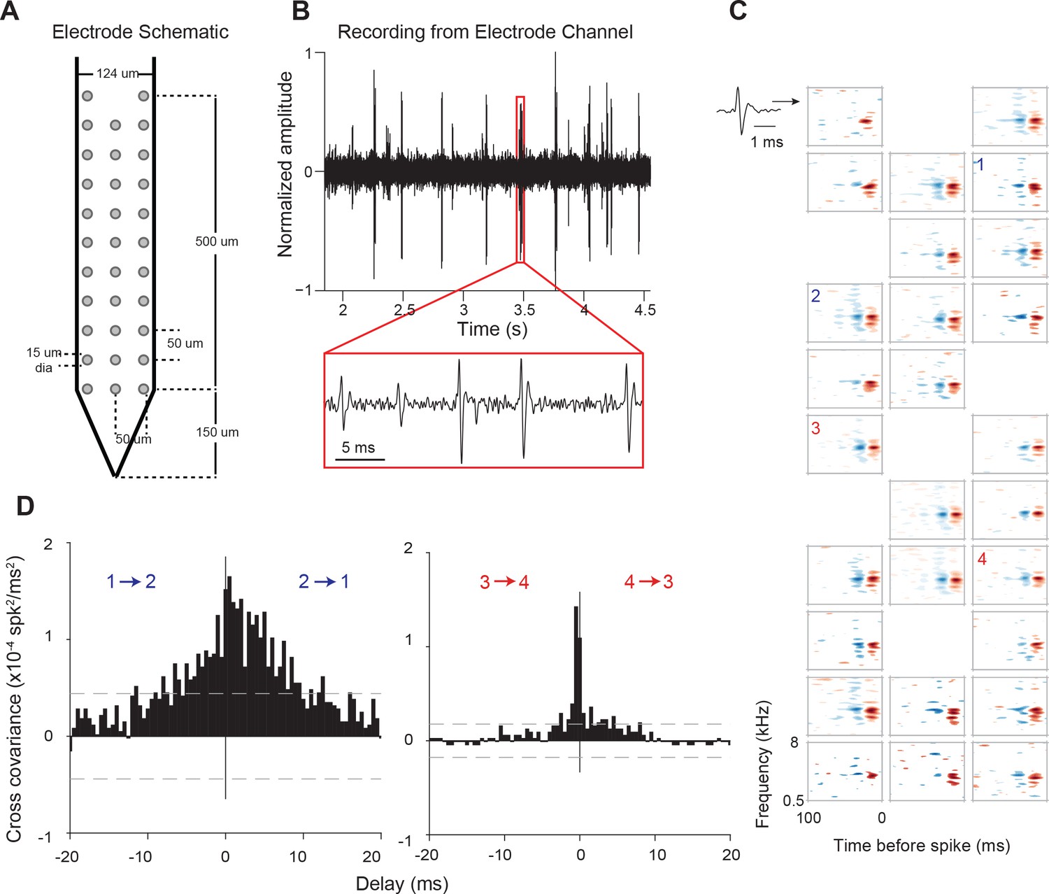
Electrode used, sample recording, STRFs, and PWCs.
(A) Electrode schematic. (B) Sample recording from one electrode channel. (C) Sample STRFs obtained after spike sorting. Numbers 1–4 indicate the positions and STRFs of pairs of neurons whose PWCs are plotted in (D). (D) Example PWCs from two pairs of neurons (1–2 and 3–4). Neurons 3 and 4 exhibit a sharper PWC than neurons 1 and 2 despite having approximately similar STRFs and pairwise distances. Dashed lines represent 99% confidence intervals.
Figure 2
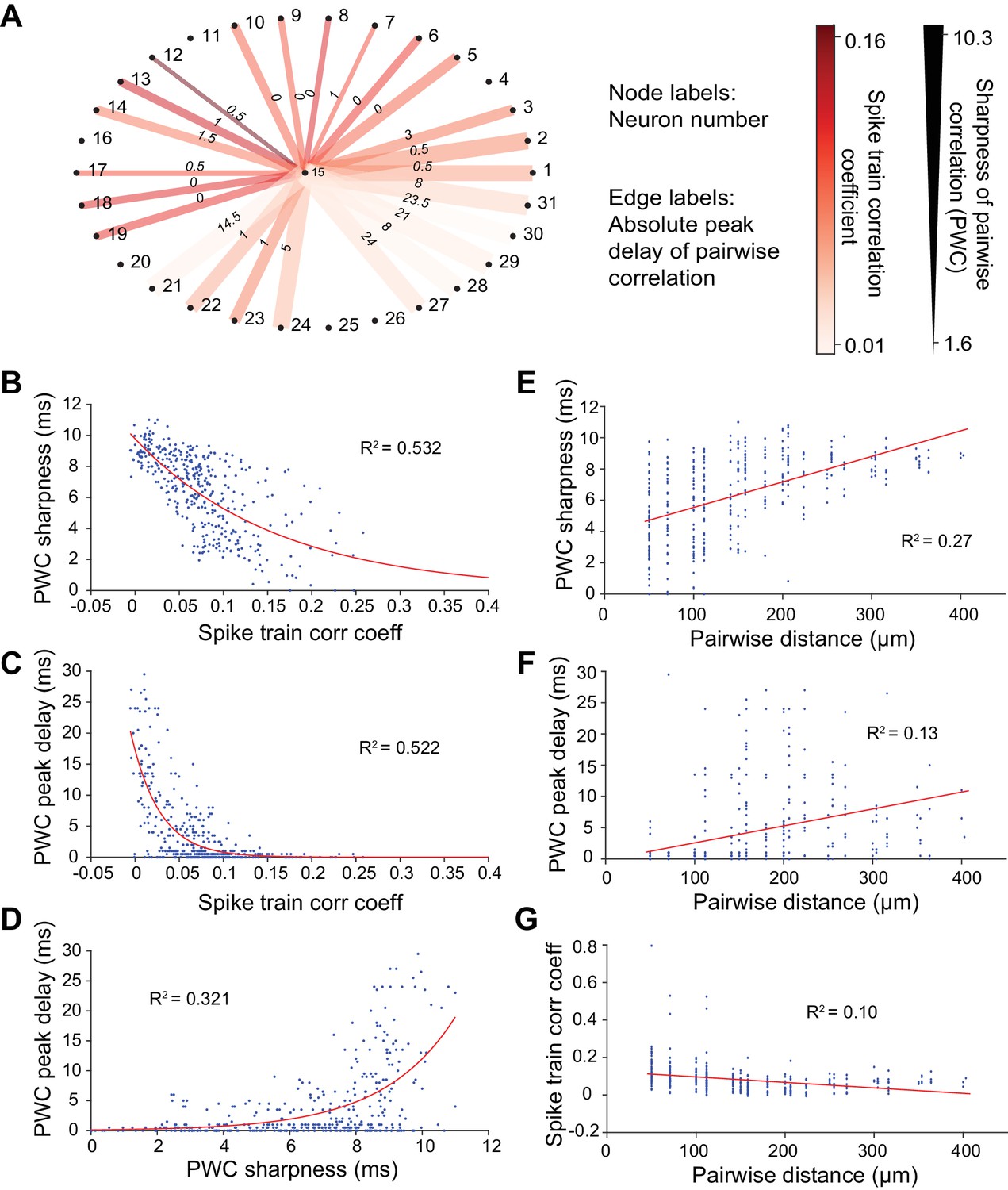
Methods for calculating neuronal correlation.
(A) An example neuron’s (#15) correlation with other neurons in a dataset of 31 neurons measured in three different ways. The node labels (outer circle numbers) represent the neuron numbers. The edge labels (inner circle numbers) represent the absolute peak delay of the pairwise correlations (PWCs). The color of the edges represents the spike train correlation coefficient (Pearson’s correlation) between pairs of neurons. The thickness of the edges represents the sharpness of the PWCs (see Figure 6G–I for an illustration of how this is computed). (B) Sharpness of PWCs against spike train correlation coefficient. (C) Peak delay of PWCs against spike train correlation coefficient. (D) Peak delay against sharpness of PWCs. All measures of correlation are highly correlated with one another. (E–G) Sharpness of PWCs (E), peak delay of PWCs (F) and spike train correlation coefficient between pairs of neurons (G) against pairwise distance. Pairwise distance explains only a small fraction of the variance seen in the different measures of correlation between pairs of neurons.
Figure 3
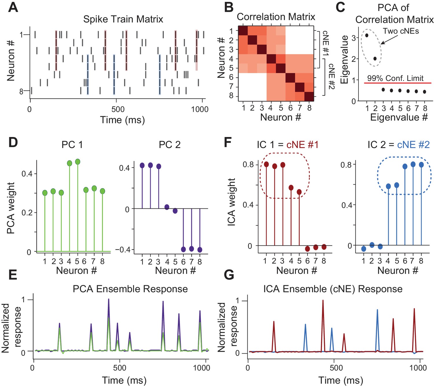
Simulated data illustrating the coordinated neuronal ensemble (cNE) detection algorithm.
(A) Raster of the simulated data. cNE #1 consists of neurons 1 to 5 while cNE #2 consists of neurons 5 to 8. Neurons 4 and 5 belong to both cNEs. Coincident spiking events between neurons in cNE #1 and cNE #2 are highlighted in red and blue respectively. (B) Correlation matrix of spike train matrix from (A). (C) Eigenvalues from applying PCA to the correlation matrix. The top two eigenvalues are significant and represent the number of cNEs. (D) The eigenvectors (or principal components, PCs) corresponding to the two significant eigenvalues from (C). The PCs do not represent the two cNEs denoted in (A) and (B). (E) Ensemble responses calculated from the projection of the PCs onto the spike train matrix. The PCA ensembles do not separate the activities of cNE #1 and #2 shown in (A). (F) Independent components (ICs) obtained after applying ICA to the two significant eigenvectors from (C). The ICs accurately represent the two cNEs denoted in (A) and (B). (G) Ensemble responses calculated from the projection of the ICs onto the spike train matrix. The ICA ensembles successfully resolve the activities of cNE #1 and #2 shown in (A).
Figure 4 with 3 supplements
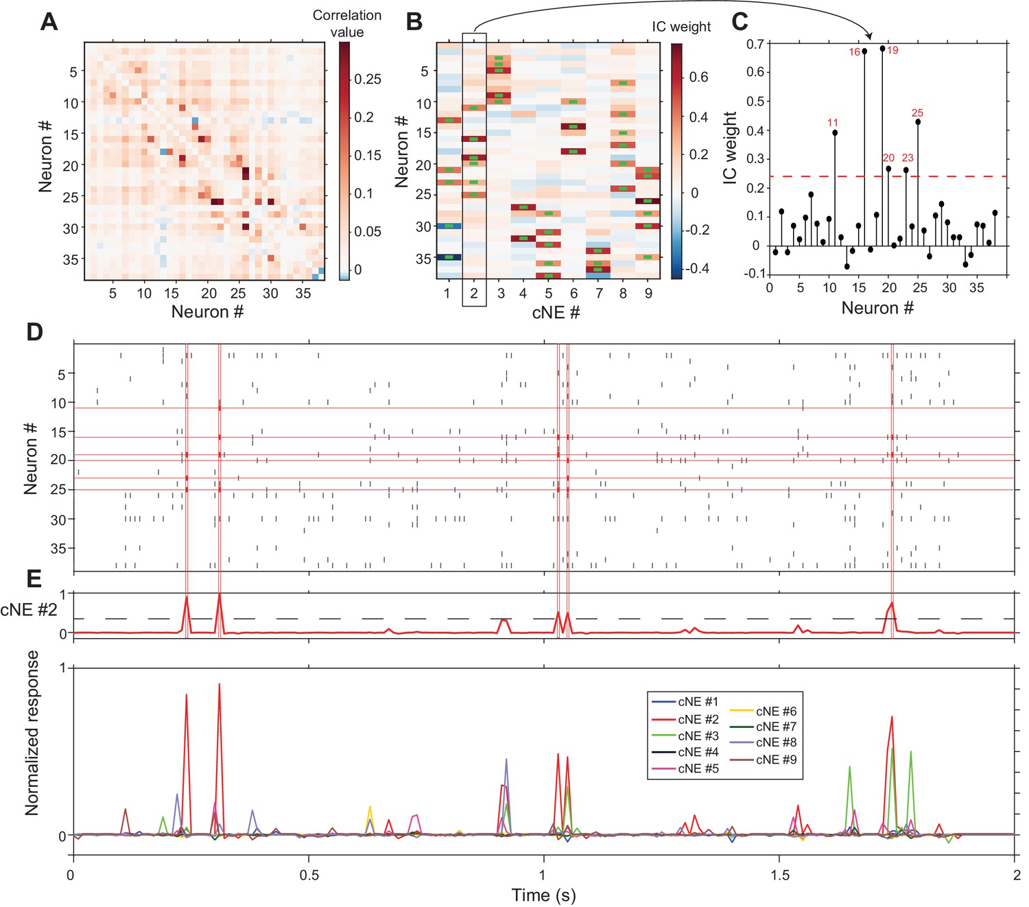
cNE detection algorithm for AI neurons.
(A) Correlation matrix of spike train matrix from (D). The diagonal has been set to 0. (B) IC weight for each neuron in each cNE. Each column represents one cNE; each row represents one neuron. The IC weight represents the contribution of each neuron to each cNE. The green bars represent neurons that are members of a cNE. (C) IC 2 (cNE #2). The red dashed line is the threshold for cNE membership determined by Monte-Carlo methods. The red numbers are the numbers of neurons that are members of the cNE. (D) Spike raster of 2 s of real data. Spikes that contribute to instances of cNE #2 activity in (E) are in red. (E) (top) Trace of cNE #2 activity. The black dashed line represents the threshold for cNE #2 activity estimated via Monte Carlo methods. Peaks that cross the threshold correspond to the coincident neuronal spikes highlighted in red in (D). (bottom) Activity traces of the 9 cNEs recovered from this dataset.
Figure 4—figure supplement 1
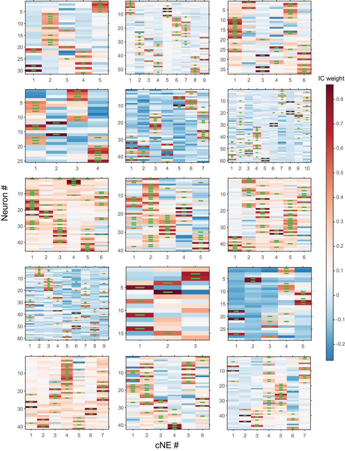
IC weights for each neuron in each cNE for all datasets used (other than the one shown in Figure 4).
Green bars represent neurons that belong to a particular cNE.
Figure 4—figure supplement 2
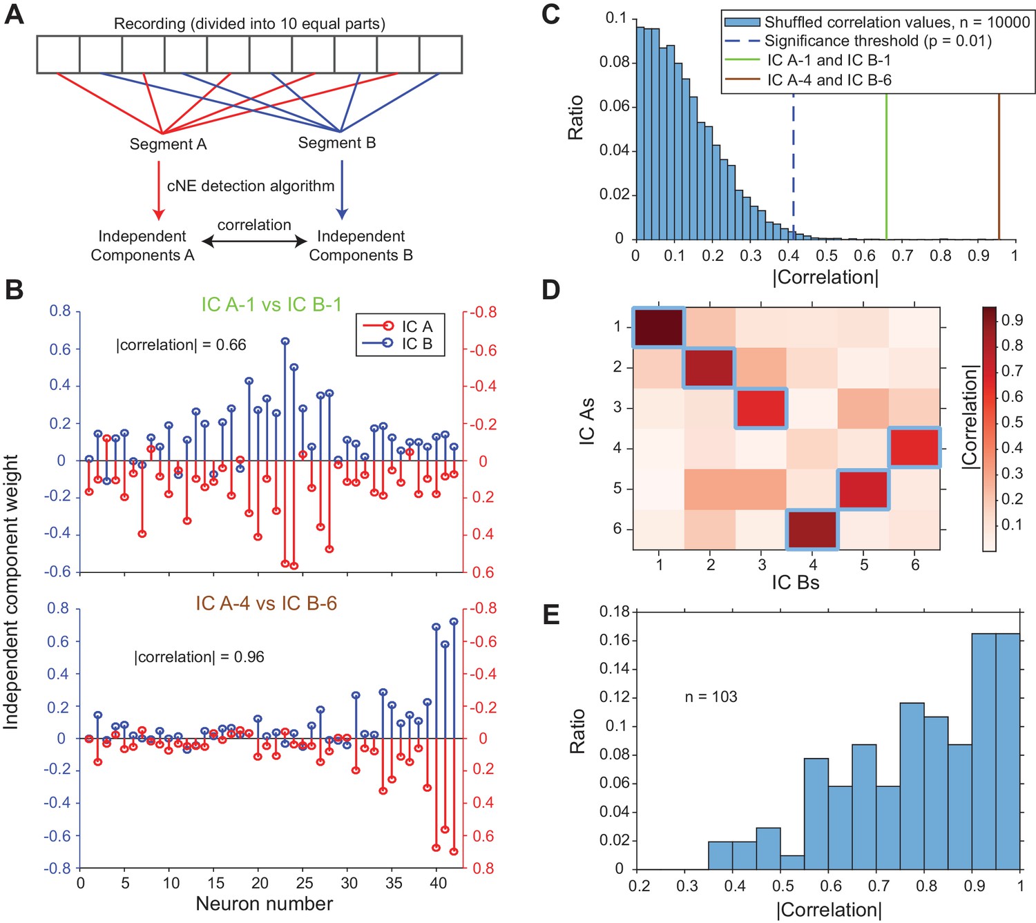
Detected cNEs are stable throughout the recording.
(A) Diagram illustrating how independent components (ICs) of two segments were calculated and compared. (B) Example pairs of ICs from one penetration. (top) Example of a pair of ICs with an absolute correlation value of 0.66. Almost all of the neurons with high weights were preserved and the low correlation value can be attributed to the noise in the neurons with low weights. (C) The two pairs of IC examples in (B) were significantly matched. See text for how the null distribution (blue bars) were calculated. Setting a significant threshold of p = 0.01 for the null distribution (blue dashed line), both comparisons in (B) were significantly matched (green and brown solid lines). (D) Absolute correlation values between the weights of IC A and IC B in one penetration (that includes the two examples in (B)). Correlation values enclosed by blue squares indicate the correlation values that are higher than the significance threshold in (C). (E) Significant correlation values obtained across all penetrations. Approximately 96% of IC As and IC Bs had significant matches.
Figure 4—figure supplement 3
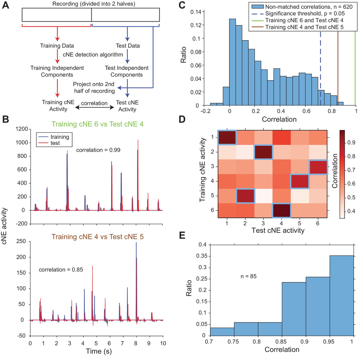
Detected cNEs are stable throughout the recording.
(A) Diagram illustrating how training cNE and test cNE activities were calculated and compared. (B) 10-s snippets of example pairs of training/test cNE activities from one penetration. Test cNE activity was offset by 50 ms for illustration purposes. (C) Correlation values between non-matched pairs, which are non-maximum values for each column and row (values not surrounded by blue squares in the example in (D)), of training and test cNE activities. The significance threshold for matched pairs (maximum correlation value in each column and row; blue squares in the example in (D)) was set at p = 0.05 (blue dashed line). The green and brown solid lines represent the correlation values of the matched examples in (B) and are significant. (D) Correlation values between the training and test cNE activities in one penetration (including the two examples in (B)). Correlation values enclosed by blue squares indicate the correlation values that are higher than the significance threshold in (C). (E) Significant correlation values across all penetrations. There were 102 training cNEs and approximately 83% of them had significant matches to the test cNEs.
Figure 5
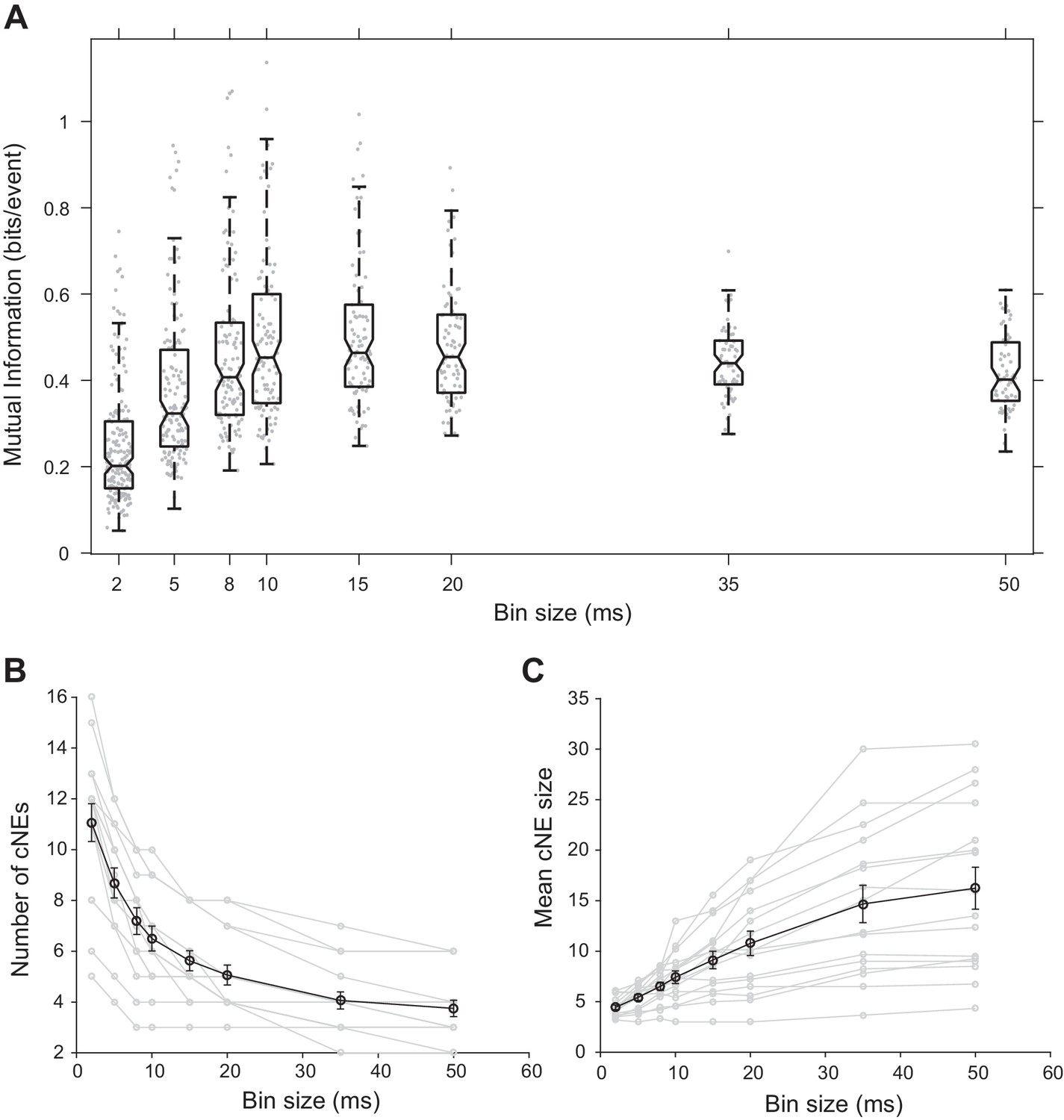
Effect of bin size on cNE properties.
(A) Mutual information between cNE STRFs and the stimulus for different bin sizes. The highest mutual information occurred for bin sizes of approximately 10 to 15 ms. (B) Number of detected cNEs decreases with increasing bin size. (C) Mean cNE size increases with increasing bin size.
-
Figure 5—source data 1
Example studies that define neuronal synchrony using different methods in different brain areas.
The temporal resolution at which synchrony is defined ranges from 5 ms to 1.4 s. Legend for brain areas – A1: primary auditory cortex, AC: auditory cortex, ACC: anterior cingulate cortex, BF: basal forebrain, DG: dentate gyrus, lAG: lateral agranular cortical area, LPFC: lateral prefrontal cortex, M1: primary motor cortex, mAG: medial agranular cortical area, mPFC: medial prefrontal cortex, PAF: posterior auditory field, PP: posterior parietal cortex, PrV: principal trigeminal brainstem nucleus, S1: primary somatosensory cortex, V1: primary visual cortex, Vg: trigeminal ganglion, VPM: ventral posterior medial thalamus.
- https://doi.org/10.7554/eLife.35587.010
Figure 6 with 1 supplement
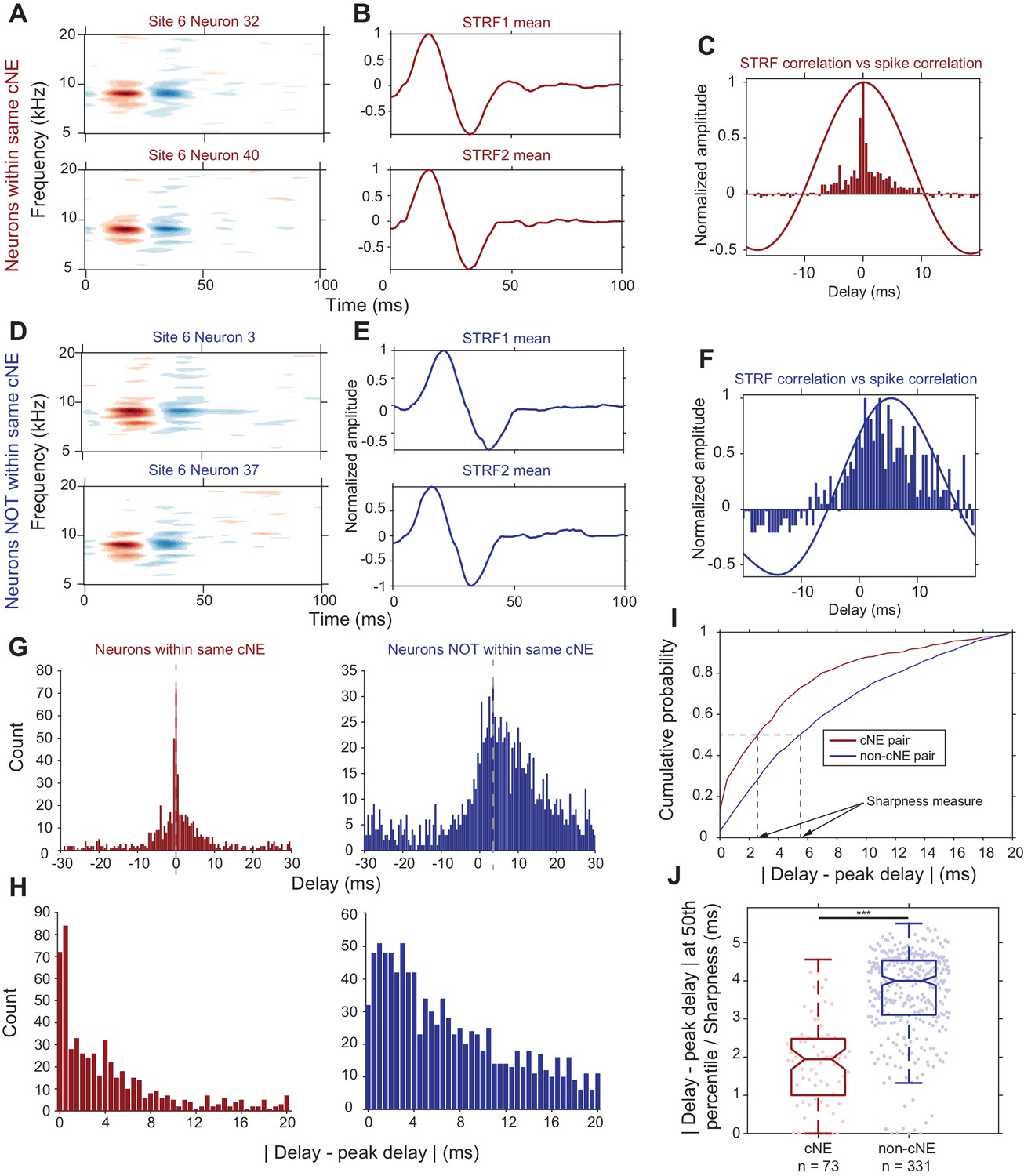
Synchrony between cNE members cannot be fully explained by receptive field overlap.
(A–C) Sample data for two neurons within the same cNE. (D–F) Sample data for two neurons not within the same cNE (but from the same recording). (A, D) STRFs for the two pairs of neurons. (B, E) Mean temporal profiles of each STRF in (A, D), obtained by averaging across the frequency axis of STRFs at every point on the time axis. (C, F) Comparisons between STRF PWCs and spike train PWCs. Neurons within the same cNE exhibit sharper spike train PWCs than STRF PWCs. Neurons not within the same cNE exhibit spike train PWCs that are as wide as their STRF PWCs. (G–I) Method for calculating sharpness of a spike train PWC. (G) Non-normalized spike train PWCs from (C) and (F). Grey dashed lines mark the peak delay (peaks of PWCs). (H) PWCs folded around their peak delays (grey dashed lines in (G)). (I) CDFs of the distributions in (H). Black dashed lines represent the time from the peak delay at the median of the distribution, which are the sharpness values for the two example PWCs in (G). (J) Sharpness comparisons for one penetration. Spike train PWCs of neurons within the same cNE are sharper than those of neurons not within the same cNE. ***p < 0.001, Mann-Whitney U test.
Figure 6—figure supplement 1
Comparison of sharpness of PWC functions of pairs within the same cNE against that of pairs not within the same cNE for all datasets (other than the one shown in Figure 6J).
For all comparisons, the sharpness values for cNE pairs were significantly less than that for non-CNE pairs (p < 0.001, Mann-Whitney U test).
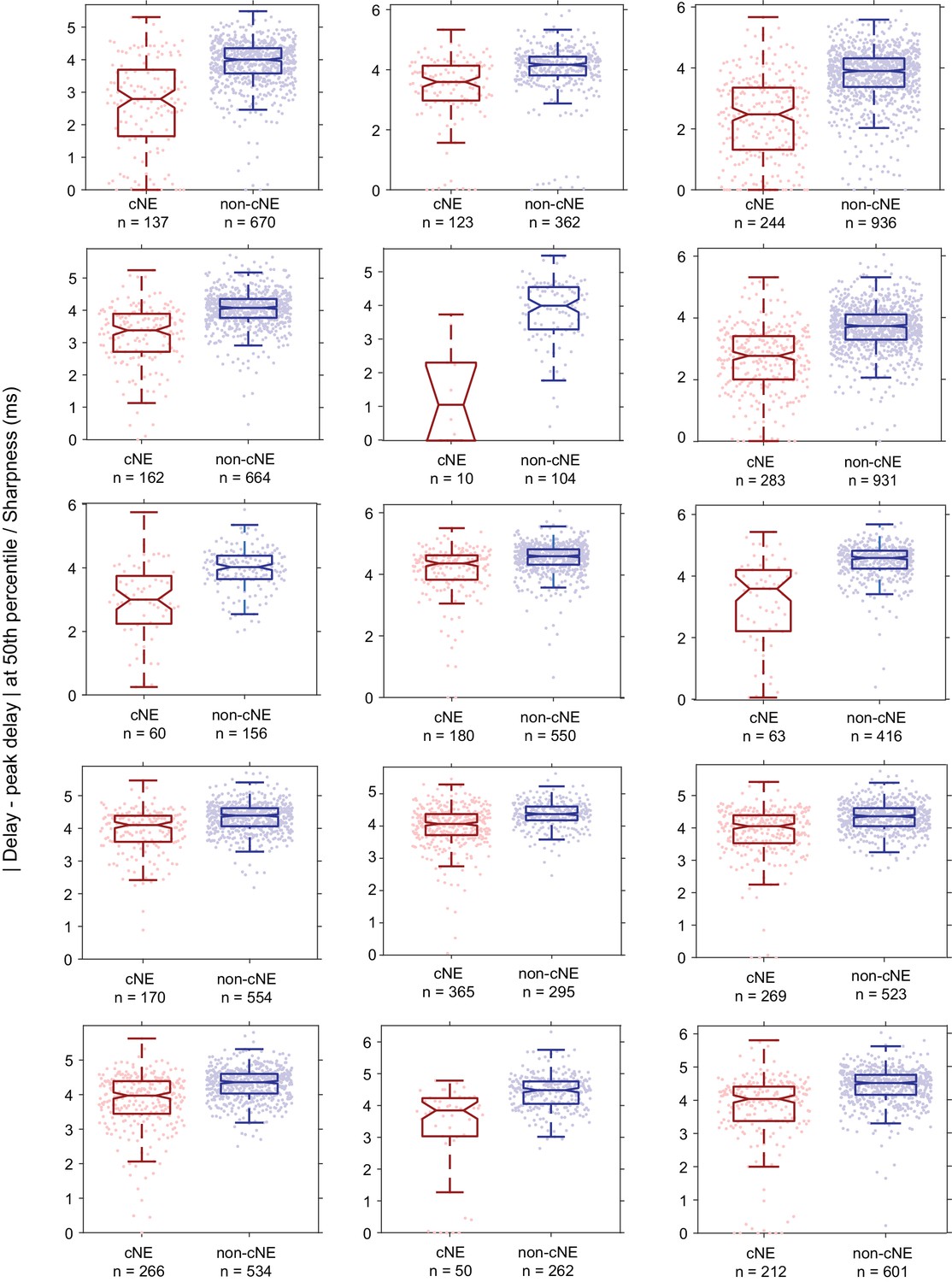
Figure 7
Properties of cNEs computed using 10-ms time bins.
(A) Number of cNEs detected increases with the number of neurons recorded. (B) Mean cNE size increases with the number of neurons recorded. (C) Most neurons recorded (~68%) belong to only 1 cNE. A small subset of neurons (~9%) did not belong to any cNE. ~23% of neurons belonged to multiple cNEs. (D) Pairwise distances between neurons in the same cNE. Most pairs of neurons in the same cNE (~82%) were recorded within <200 μm of each other. (E) Depth of cNEs, of neurons within cNEs and of all isolated neurons. The depth of each cNE was calculated by taking the median depth of each cNE’s member neurons. The depth of neurons within cNEs is the depth of all neurons found in at least one cNE, i.e. all recorded neurons except those found in the 0 bin in (C). The dashed line indicates the putative boundary between layers II/III and layer IV based on Szymanski et al., 2009. There was no depth bias for cNE neurons, that is the distributions of the depth of cNE members and that of all recorded neurons were similar. (F) cNE span, determined by the difference between the maximum and minimum depth of member neurons in each cNE. Most cNEs (~70%) had a span of 200 μm or less.
Figure 8
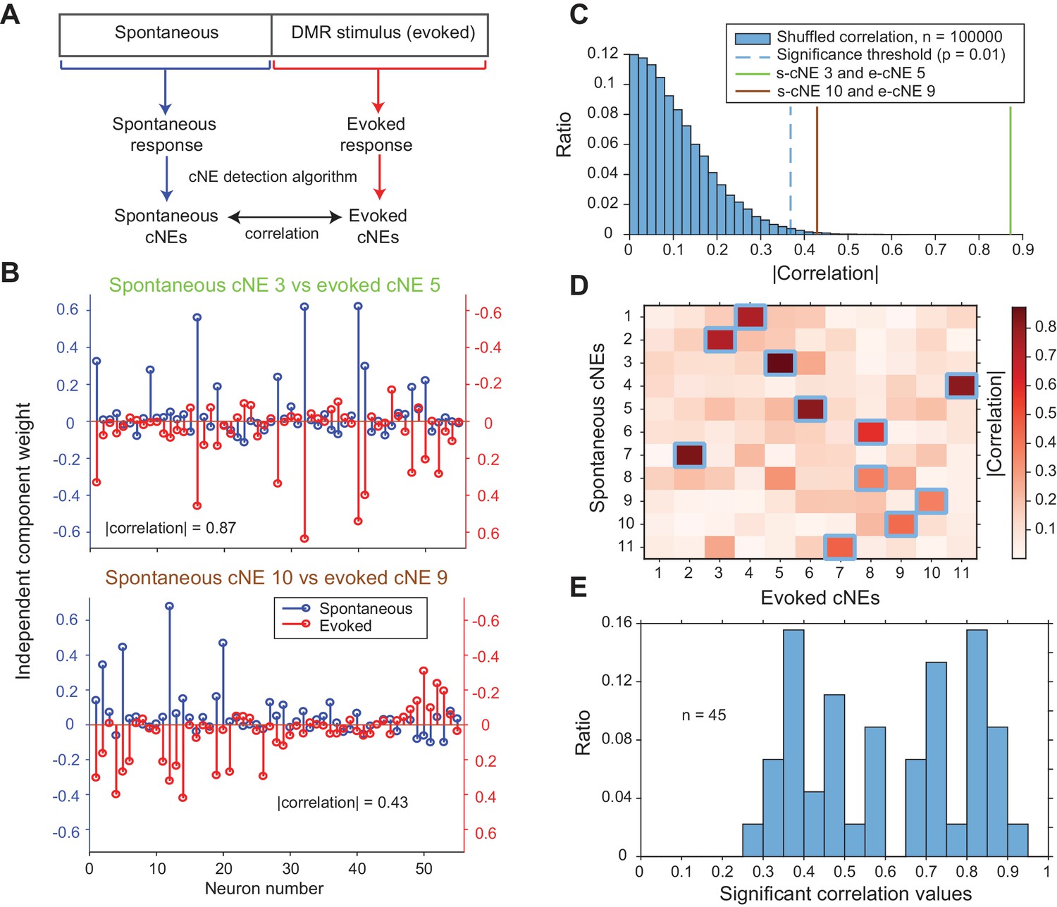
cNEs are highly preserved across spontaneous and evoked activity.
(A) Illustration of the procedure for comparing spontaneous cNEs with evoked cNEs. (B) Examples of pairs of spontaneous-evoked cNEs from one penetration. (top) A pair of cNEs with an absolute correlation value of 0.87, implying that this particular cNE was highly preserved regardless of the presence of a stimulus. (bottom) A pair of cNEs with a lower absolute correlation value of 0.43. Almost all of the neurons with high weights were preserved and the low correlation value can be attributed to the noise in the neurons with low weights. (C) The two pairs of cNE examples in (B) were significantly matched. See text for how the null distributions (blue bars) were calculated. Setting a significant threshold of p = 0.01 for the null distribution (blue dashed line) revealed that both comparisons in (B) were significantly matched (green and brown solid lines). (D) Absolute correlation values between the weights of spontaneous and evoked cNEs in one penetration (that includes the two examples in (B)). Correlation values enclosed by blue squares indicate the correlation values that are higher than the significance threshold in (C). (E) Significant correlation values across all penetrations with contiguous spontaneous and DMR-evoked recordings. Approximately 72% of cNEs (both spontaneous and evoked) had significant matches.
Figure 9 with 2 supplements
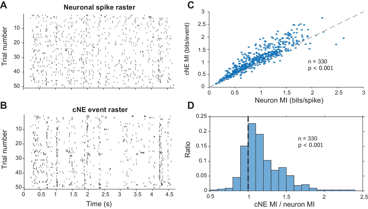
Mutual information (MI) carried by patterns of cNE events is higher than MI carried by patterns of single neuron spikes.
(A) Raster for neuronal spikes over 50 presentations of a ~5-s long DMR or RN stimulus. (B) Raster for cNE events over 50 presentations of the stimulus. The neuron in (A) is a member of the cNE in (B). Random sampling was used to ensure equivalent spike or event counts for each comparison. (C) Population data for cNE MI against single neuron MI. cNE MI was significantly higher than that of the cNE’s constituent neurons. (D) cNE MI/neuron MI. Wilcoxon signed-rank test was used in (C) and (D).
Figure 9—figure supplement 1
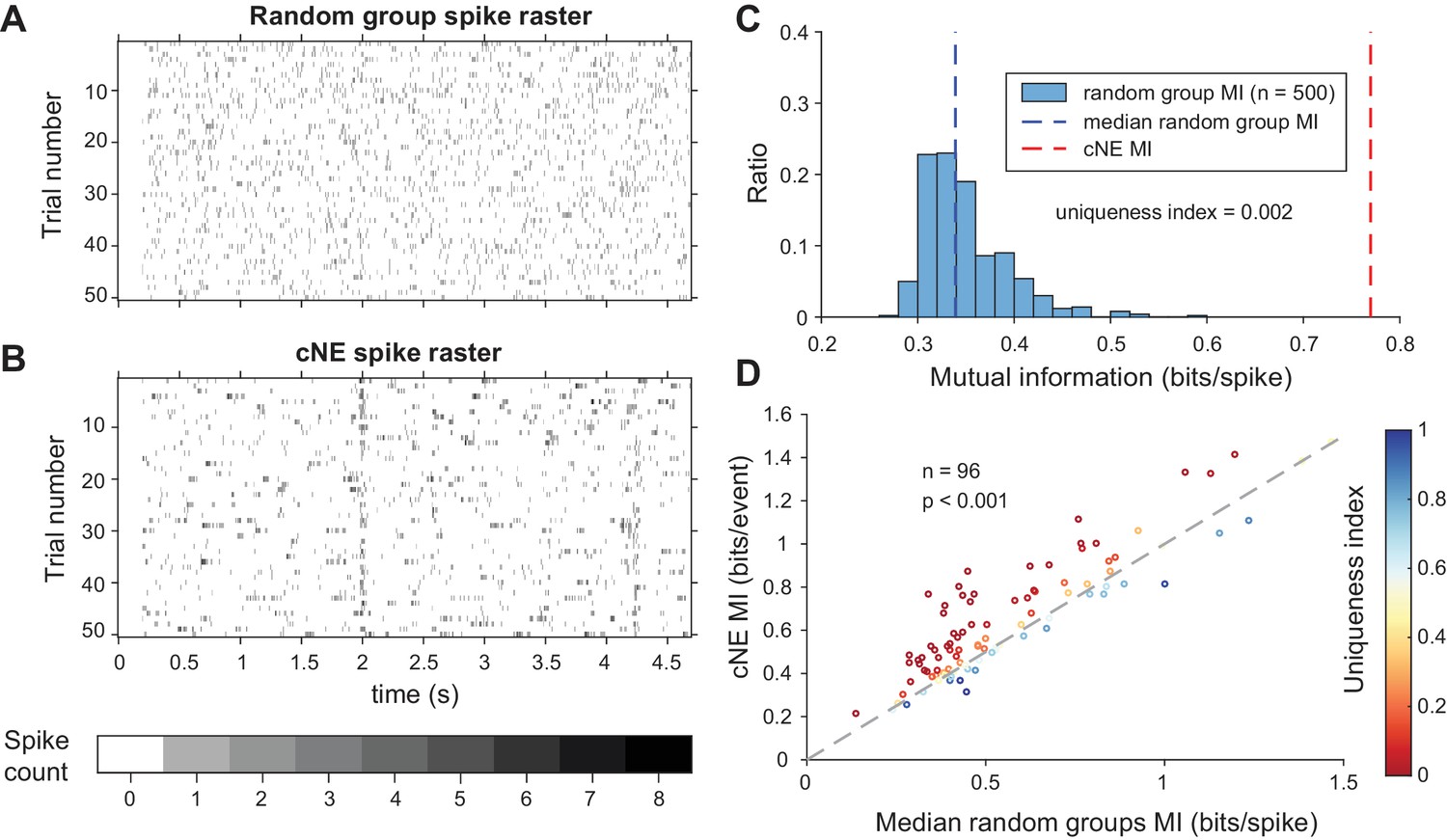
Mutual information (MI) carried by patterns of cNE members’ spikes is higher than that of random groups of neurons.
(A) Raster for the summed spikes of a random group of neurons over 50 presentations of a ~5-s long DMR or RN stimulus. Each random group of neurons has one neuron in common with the cNE it is being compared to in (B). (B) Raster for the summed spikes of all members of a cNE over 50 presentations of the stimulus. Random sampling was used to ensure equivalent spike counts for each comparison. (C) MI values for 500 randomly chosen groups (blue bars) and cNE (red dashed line), for the example in (B). The uniqueness index is the proportion of the entire distribution (blue bars and red dashed line; n = 501) that is greater than or equal to the cNE MI value (red dashed line). The minimum possible uniqueness index is therefore 0.002. (D) Population data for cNE MI against the median of the random group MI (blue dashed line in (C)). cNE MI was significantly higher than the MI for random groups of neurons. The uniqueness index for each cNE-random group comparison is colored according to the displayed color bar. Wilcoxon signed-rank test was used in (D).
Figure 9—figure supplement 2
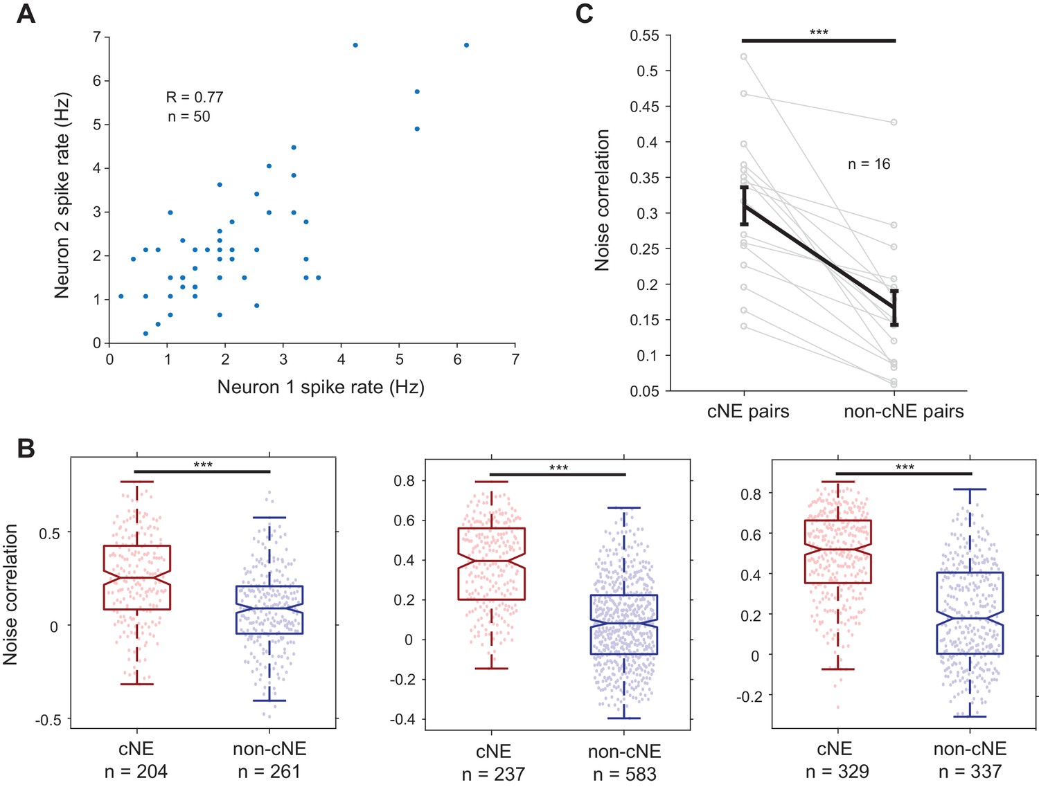
Noise correlations between cNE pairs were higher than those between non-cNE pairs.
(A) Example spike rates for a pair of neurons over 50 trials of the short, repeated stimulus. The noise correlation was calculated as the Pearson’s correlation coefficient (R) between the two neurons’ spike rates over different trials. (B) Examples of raw noise correlation data from 3 of the 16 recordings. All recordings had noise correlations between cNE pairs that were significantly higher than noise correlations between non-cNE pairs. (C) Summary figure for all 16 recordings. The median noise correlations for each group and recording are plotted. ***p < 0.001, Mann-Whitney U-test was used for (B), paired t-test was used for (C).
Figure 10 with 1 supplement
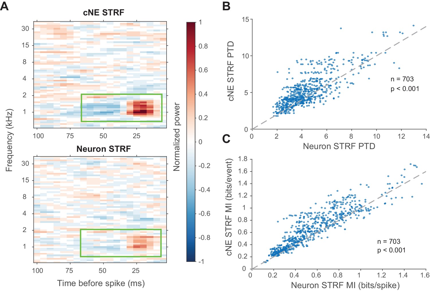
cNE STRFs have enhanced features compared to STRFs of member neurons.
(A) Example comparison between a cNE’s STRF (top) and a member neuron’s STRF (bottom). Random sampling was done to estimate STRFs with equivalent spike/event counts. The color scales for the sample STRFs have been normalized. The cNE STRF has stronger excitatory and inhibitory subfields than the neuronal STRF (highlighted by green boxes). (B) Over the entire population, cNE STRFs had a higher peak-trough difference (PTD) than neuronal STRFs. PTD was the difference between the highest and lowest STRF values, divided by the number of spikes/events. (C) Similarly, cNEs had higher mutual information (MI) between their STRFs and single events than neurons had between their STRFs and single spikes. Wilcoxon signed-rank test was used in (B) and (C).
Figure 10—figure supplement 1
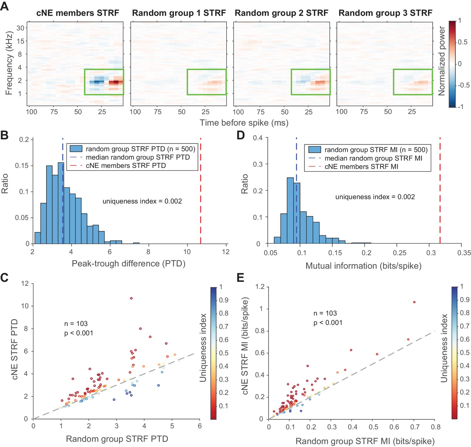
cNE members have multi-unit STRFs with enhanced features compared to the multi-unit STRFs of random groups of neurons.
(A) Sample of a comparison between the multi-unit STRF of members of a cNE (left-most) and the multi-unit STRFs of random groups of neurons the same size as the cNE. The number of spikes used to calculate the STRFs was equalized via random sampling. The color scales for the sample STRFs have also been normalized. The STRF for cNE members shows stronger excitatory and inhibitory subfields than the STRFs for random groups (highlighted by green boxes). (B) Peak-trough difference (PTD) values for 500 iterations of random groups (blue bars) and cNE (red dashed line), for the example in (A). The uniqueness index is the proportion of the entire distribution (blue bars and red dashed line; n = 501) that is greater than or equal to the cNE PTD (red dashed line). The minimum possible uniqueness index is therefore 0.002. (C) Population data for cNE PTD against the median of random group PTD (blue dashed line in (B)). cNE PTD was significantly higher than that of random groups of neurons. The uniqueness index for each cNE-random group comparison is colored according to the displayed color bar. (D) Similar to (B), but for mutual information (MI) between the multi-unit STRFs and single spikes. (E) Similar to (C), but for MI. cNE MI was significantly higher than that of random groups of neurons. Wilcoxon signed-rank test was used in (C) and (E).
Figure 11 with 4 supplements
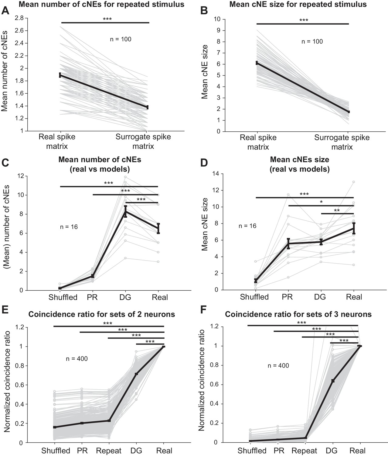
Receptive field similarity is insufficient to explain the coincident spiking between neurons in the same cNE.
(A) The number of cNEs identified in ‘real’ spike train matrices is significantly higher than that of ‘surrogate’ spike train matrices. (B) Mean size of cNEs identified in ‘real’ spike train matrices is significantly larger than that of ‘surrogate’ spike train matrices. See Figure 11—figure supplement 1 for details on how the spike train matrices were constructed. Each paired dataset represents one unique combination of 15 neurons. (C) The number of cNEs identified in the ‘real’ data is significantly higher than that of the ‘shuffled’ and ‘PR’ models, but is significantly lower than that of the ‘DG’ model. (D) The mean size of cNEs identified in the ‘real’ data is significantly larger than that of the ‘shuffled’, ‘PR’ and ‘DG’ models. See Figure 11—figure supplement 2A for how the ‘PR’ model was computed. Each dataset represents the mean number of cNEs and the mean cNE size for one recording over 200 iterations. (E, F) The coincidence between neurons from different repeats of the same stimulus (’repeat’), or from the ‘shuffled’, ‘PR’ and ‘DG’ models is significantly less than the coincidence seen between neurons from the same cNE in the ‘real’ data. See Figure 11—figure supplement 4 for how the coincidence ratio (CR) was calculated. Each dataset represents a unique combination of 2 or three neurons and was normalized by the CR between neurons from the ‘real’ spike matrix. Sets of more than three neurons had coincidence ratios that were close to zero for most models and are not shown. *p < 0.05, **p < 0.01 ***p < 0.001, paired t-test with Bonferroni correction.
Figure 11—figure supplement 1
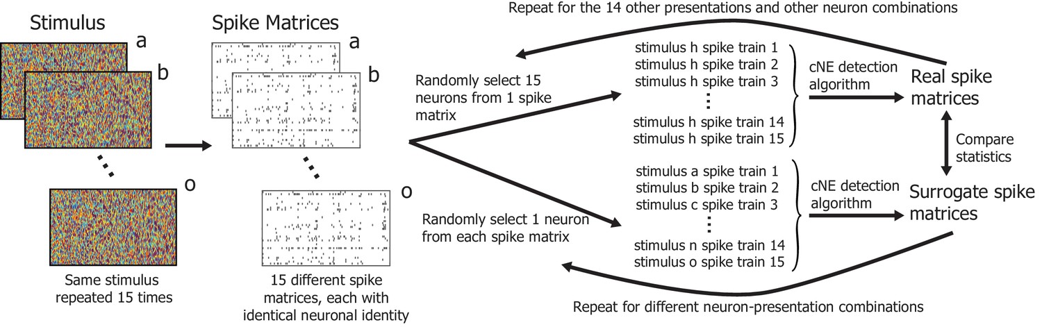
Illustration of the process of constructing spike trains from different presentations of the same stimuli to obtain ‘real’ and ‘surrogate’ spike matrices.
The statistics of these spike matrices are presented in Figure 11A and B.
Figure 11—figure supplement 2
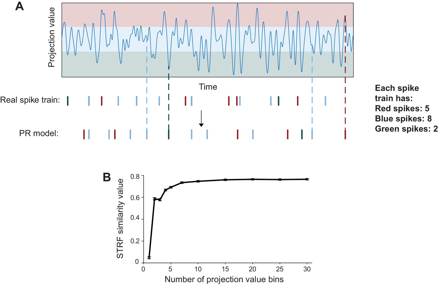
Method for the ‘preserved receptive field’ (‘PR’) model.
(A) Illustration of how the ‘PR’ model was computed. The similarity between stimulus segments and each neuron’s receptive field (projection value) was calculated and binned. The red, blue and green shades represent the three bins in this simple illustration, even though 15 bins were used in the actual model. The spikes, each belonging to a projection value bin (and colored correspondingly) were then randomly reassigned to another time bin within the same projection value. (B) STRF similarity values between STRFs obtained from the ‘PR’ model and the STRFs of the ‘real’ spike trains against the number of projection value bins used in computing the ‘PR’ model. The similarity values plateaued after 15 projection value bins, justifying the use of 15 projection value bins.
Figure 11—figure supplement 3
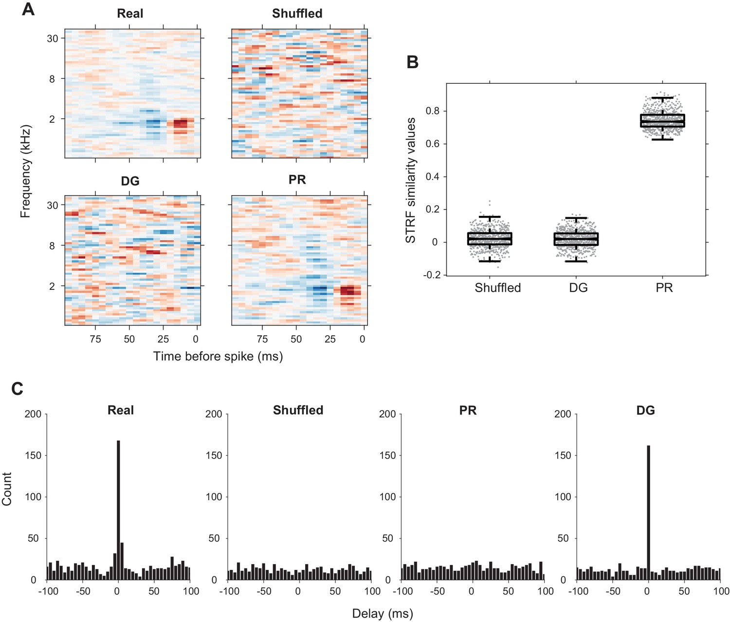
Verification of the ‘shuffled’, ‘PR’, and ‘DG’ models.
(A) Sample STRFs for one neuron from the ‘real’ spike train, ‘shuffled’, ‘DG’ and ‘PR’ models. The ‘PR’ model has similar STRFs to that of the ‘real’ spike trains while the ‘shuffled’ and ‘DG’ models do not. (B) STRF similarity values between neuronal spike trains from the ‘shuffled’, ‘DG’ and ‘PR’ models and the ‘real’ spike trains. The STRFs obtained from the ‘PR’ model spike trains were highly similar to the STRFs obtained from ‘real’ spike trains, while the ‘shuffled’ and ‘DG’ models have STRFs that are uncorrelated with the ‘real’ STRF. (C) PWC functions at 5-ms temporal resolution for one pair of neurons. The correlations in the ‘shuffled’ and ‘PR’ models have been completely broken. The ‘DG’ model preserves the correlation at zero delay but not at other time delays. Using 5-ms time bins captures almost all the temporal correlations between two neurons in a real spike train.
Figure 11—figure supplement 4
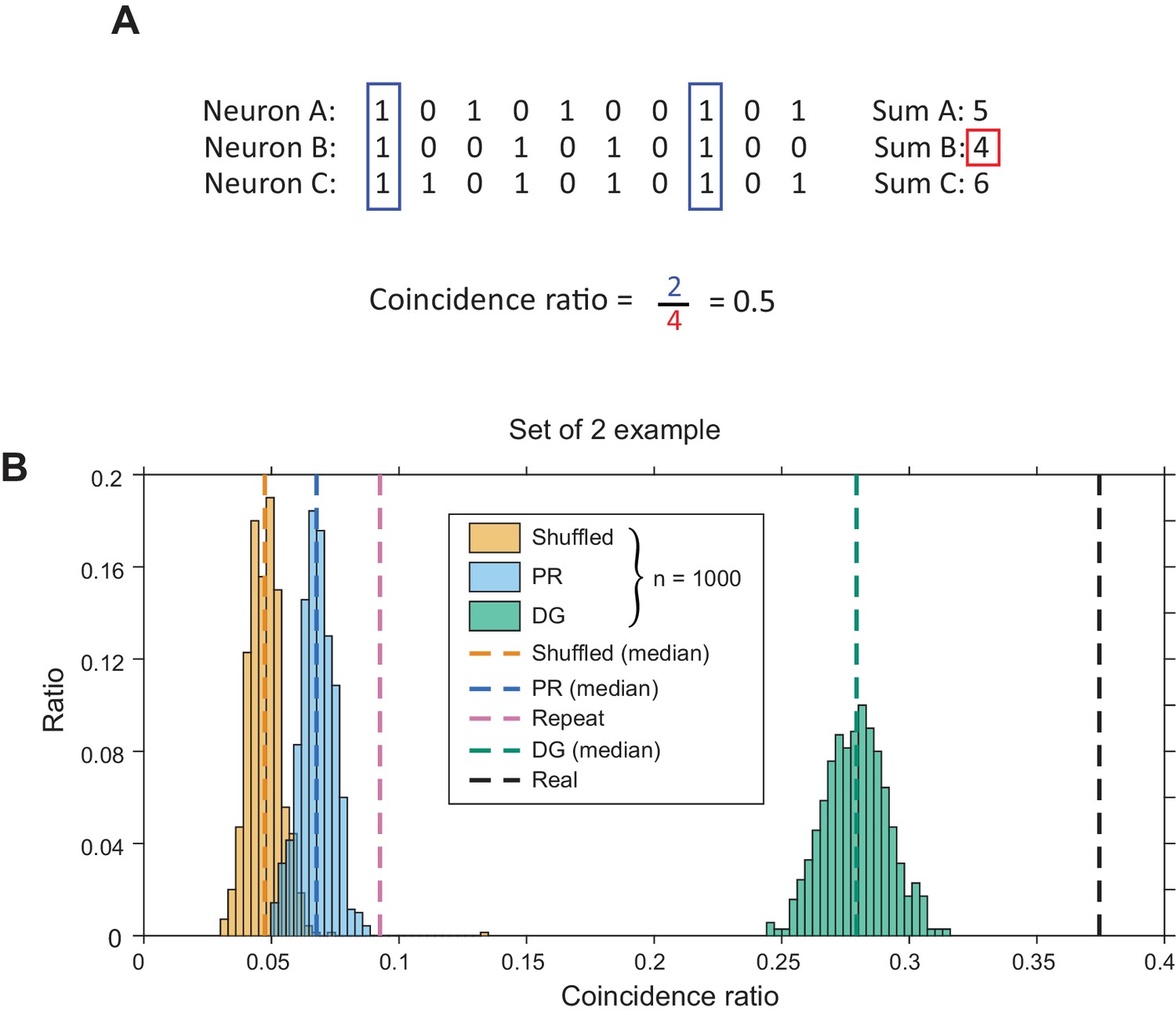
Calculation of coincidence ratio between groups of neurons in the same cNE.
(A) Illustration of how coincidence ratio (CR) was calculated for a set of 3 neurons. The maximum CR is 1 (when all neurons spike whenever the neuron with the lowest firing rate spikes) and the minimum CR is 0 (when there are no coincident bins). (B) Sample CR values for an example set of 2 neurons. The ‘repeat’ model compares two pairs of spike trains from different presentations of the same stimulus. Distributions represent 1000 iterations of the ‘shuffled’, ‘PR’ and ‘DG’ models and associated coincidence ratios. Together with ‘repeat’ and ‘real’ values, these values comprise one dataset in Figure 11E.
Additional files
-
Supplementary File 1
Details of statistical tests used in the study, including the type of statistical tests used, the sample sizes (N), and the exact p-values.
- https://doi.org/10.7554/eLife.35587.025
-
Transparent reporting form
- https://doi.org/10.7554/eLife.35587.026
Download links
A two-part list of links to download the article, or parts of the article, in various formats.
Downloads (link to download the article as PDF)
Open citations (links to open the citations from this article in various online reference manager services)
Cite this article (links to download the citations from this article in formats compatible with various reference manager tools)
Coordinated neuronal ensembles in primary auditory cortical columns
eLife 7:e35587.
https://doi.org/10.7554/eLife.35587


