Content-specific activity in frontoparietal and default-mode networks during prior-guided visual perception
- National Institutes of Health, United States
- Ghent University, Belgium
- New York University Langone Medical Center, United States
Figures
Figure 1
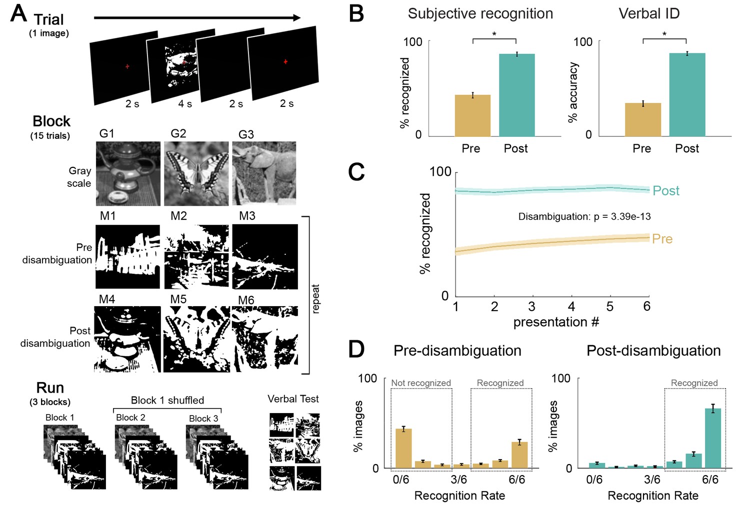
Paradigm and behavioral results.
(A) Task design, and flow of events at trial, block, and fMRI run level. Subjects viewed gray-scale and Mooney images and were instructed to respond to the question ‘Can you recognize and name the object in the image?”. Each block included three gray-scale images, three money images corresponding to these gray-scale images (i.e., post-disambiguation Mooney images), and three Mooney images unrelated to the gray-scale images (i.e. pre-disambiguation Mooney images, as their corresponding gray-scale images would be presented in the following block). 33 unique images were used and each was presented six times before and six times after disambiguation (see Materials and methods for details). (B) Left: Percentage of ‘recognized’ answers across all Mooney image presentations before and after disambiguation. These two percentages significantly differed from each other (p=3.4e-13). Right: Percentage of correctly identified Mooney images before and after disambiguation. These two percentages significantly differed from each other (p=1.7e-15). (C) Recognition rate for Mooney images sorted by presentation number, for the pre- and post-disambiguation period, respectively. A repeated-measures ANOVA revealed significant effects of the condition (p=3.4e-13), the presentation number (p=0.002), and the interaction of the two factors (p=0.001). (D) Distribution of recognition rate across 33 Mooney images pre- (left) and post- (right) disambiguation. Dashed boxes depict the cut-offs used to classify an image as recognized or not-recognized. All error bars denote s.e.m. across subjects.
Figure 2 with 4 supplements
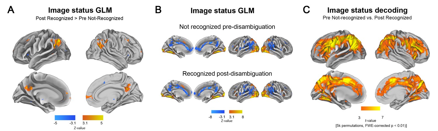
Disambiguation-induced changes in neural activity magnitude and pattern.
(A) GLM contrast related to the disambiguation effect. For each subject, the set of Mooney images that were not recognized in the pre-disambiguation period and recognized in the post-disambiguation period are used. Thus, the GLM contrast is between an identical set of images that elicit distinct perceptual outcomes. Warm colors show regions with significantly higher activity magnitudes after than before disambiguation (p<0.05, FWE-corrected). (B) Activation and deactivation maps for each condition separately (p<0.05, FWE-corrected). Top row: Activation/deactivation map corresponding to pre-disambiguation, not recognized Mooney images, as compared to baseline. Bottom row: post-disambiguation, recognized Mooney images. (C) Searchlight decoding of Mooney image status (pre-disambiguation not-recognized vs. post-disambiguation recognized). For each subject, the same set of Mooney images are included in both conditions. Results are shown at p<0.01, corrected level (cluster-based permutation test).
Figure 2—figure supplement 1
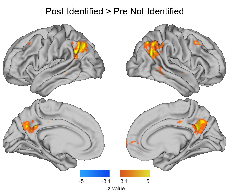
GLM results of the post-disambiguation identified >pre disambiguation not-identified contrast, based on the verbal identification responses.
For each subject, the same set of Mooney images are included in both conditions. Results were corrected for multiple comparisons using a cluster-defining threshold of z > 3.1, cluster size ≥17 voxels, corresponding to p<0.05, FWE-corrected (for details see Materials and methods, GLM analysis).
Figure 2—figure supplement 2
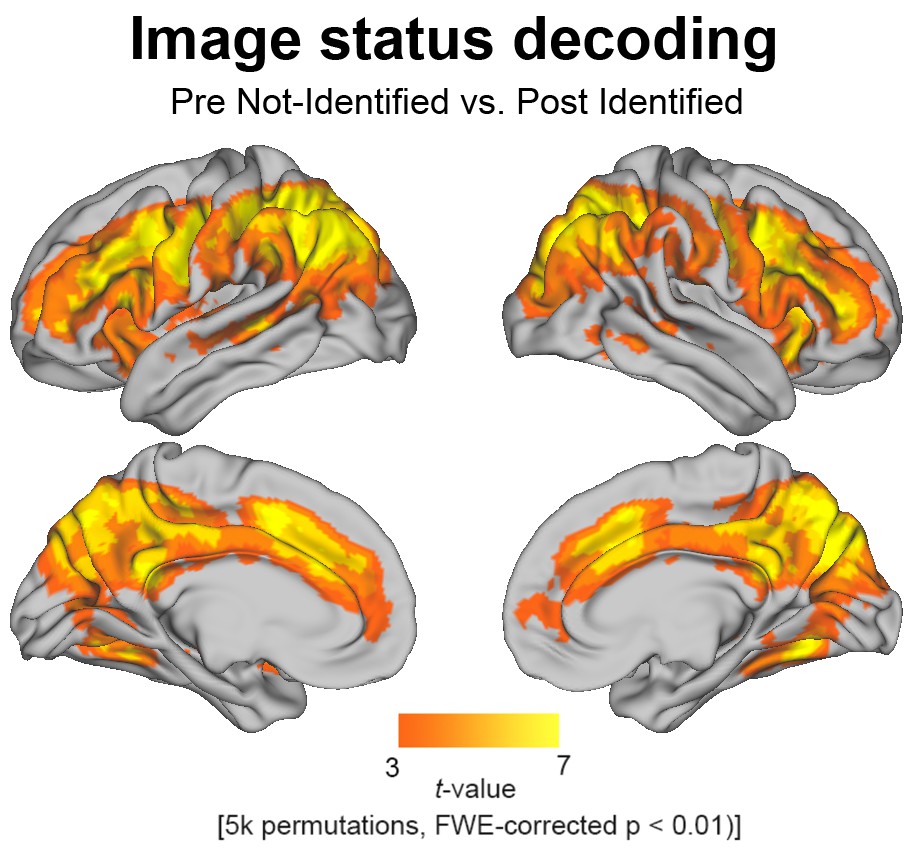
Searchlight decoding of pre-disambiguation not-identified vs post-disambiguation identified Mooney images, selected based on verbal identification responses.
For each subject, the same set of images are included in both conditions. Results were corrected for multiple comparisons using a cluster-based permutation test and thresholded at a p<0.01, corrected level (for details see Materials and methods, MVPA).
Figure 2—figure supplement 3
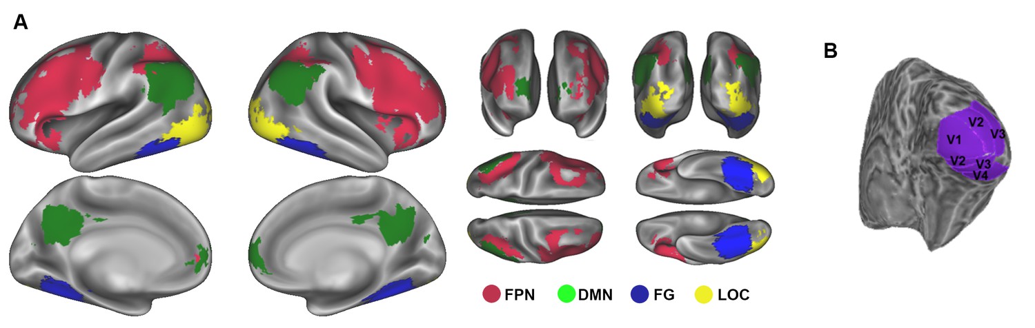
Regions of interest (ROIs) used in RSA.
(A) The FPN included the following ROIs: right frontal (14427 voxels, vx), left frontal (13383 vx), right parietal (3381 vx) and left parietal (3949 vx). The DMN included: MPFC (1135 vx), PCC (2145 vx), right lateral parietal (1469 vx) and left lateral parietal (1361 vx). Category-selective regions included the right (4572 vx) and left (4176 vx) fusiform gyrus (FG), and the right (744 vx) and left (1195 vx) lateral occipital complex (LOC). FPN ROIs were defined at the population level first and then registered back to each subject’s native space. FG ROIs were extracted from a structural atlas and registered back to each subject’s native space as well. DMN and LOC ROIs were individually defined based on each subject’s estimate of relevant GLM contrasts (see Materials and methods, ROI definition). (B) Example of single-subject early visual ROIs (right hemisphere shown). Early visual ROIs included right V1 (577 vx), left V1 (550 vx), right V2 (637 vx), left V2 (564 vx), right V3 (540 vx), left V3 (477 vx), right V4 (256 vx) and left V4 (198 vx). A retinotopic functional localizer was performed to delineate these ROIs in each subject’s native space. All voxel (vx) counts reported in parentheses were calculated in each subject’s native space, and then averaged across subjects.
Figure 2—figure supplement 4
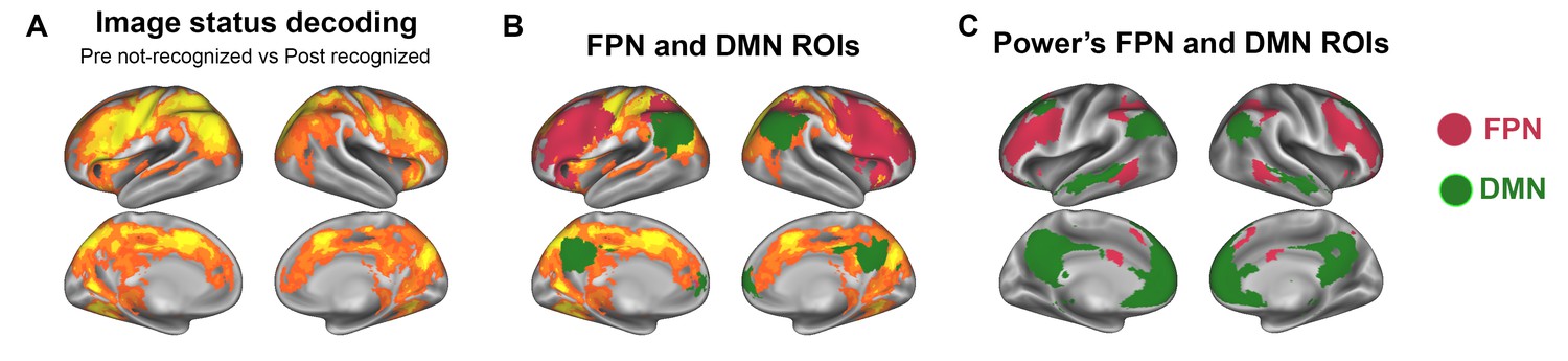
The definition of FPN ROIs from image status decoding results (for details, see Materials and methods, ROI definition).
(A) Searchlight decoding of Mooney image status, reproduced from Figure 2C on inflated cortical surface. (B) The map from A is overlaid with the FPN and DMN ROIs used in this study. These ROIs are also shown in Figure 2—figure supplement 3. (C) FPN and DMN ROIs reported in Power et al. (2011).
Figure 3 with 2 supplements
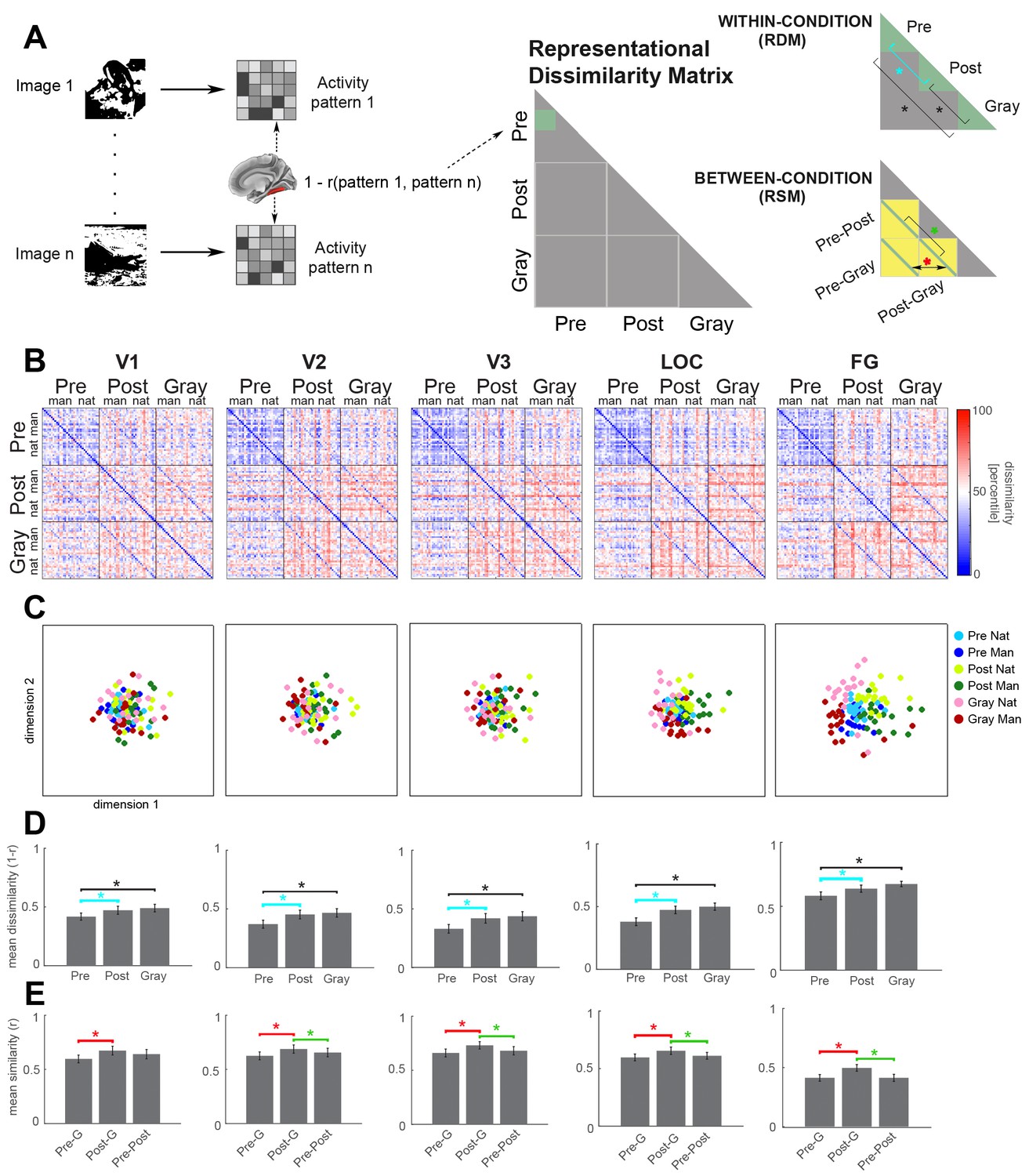
Neural representation format of individual images in visual regions.
(A) Analysis schematic. Dissimilarity (1 – Pearson’s r) between the neural response patterns to pairs of images was computed to construct the representational dissimilarity matrix (RDM) for each ROI. Two statistical analyses were performed: First (top-right panel, ‘within-condition’), mean dissimilarity across image pairs was calculated for each condition (green triangles), and compared between conditions (brackets). Cyan bracket highlights the main effect of interest (disambiguation). Second (bottom-right panel, ‘between-condition’), the mean of between-condition diagonals (green lines) was compared. For ease of interpretation, this analysis was carried out on the representational similarity matrix (RSM). Each element in the diagonal represents the neural similarity between the same Mooney image presented in different stages (Pre-Post), or between a Mooney image and its corresponding gray-scale image (Pre-Gray and Post-Gray). (B) Group-average RDMs for V1, V2, V3, LOC and FG ROIs in the right hemisphere. Black lines delimit boundaries of each condition. Within each condition, natural (‘nat’) and man-made (‘man’) images are grouped together. (C) 2-D MDS plots corresponding to the RDMs in B. Pre-disambiguation, post-disambiguation, and gray-scale images are shown as blue, yellow-green, and pink-red dots, respectively. (D) Mean within-condition representational dissimilarity between different images for each ROI, corresponding to the ‘within-condition’ analysis depicted in A. (E) Mean between-condition similarity for the same or corresponding images for each ROI, corresponding to the ‘between-condition’ analysis depicted in A. In D and E, asterisks denote significant differences (p<0.05, Wilcoxon signed-rank test, FDR-corrected), and error bars denote s.e.m. across subjects. Results from V4 are shown in Figure 3—figure supplement 2. Interactive 3-dimensional MDS plots corresponding to first-order RDMs for each ROI can be found at: https://gonzalezgarcia.github.io/mds.html.
-
Figure 3—source data 1
RDM for each ROI in each subject. Includes source code to perform statistical analysis and produce Figure 3 and 4.
- https://doi.org/10.7554/eLife.36068.011
Figure 3—figure supplement 1
RSA results for left hemisphere visual regions.
Same as Figure 3B–E, but for left hemisphere ROIs.
Figure 3—figure supplement 2
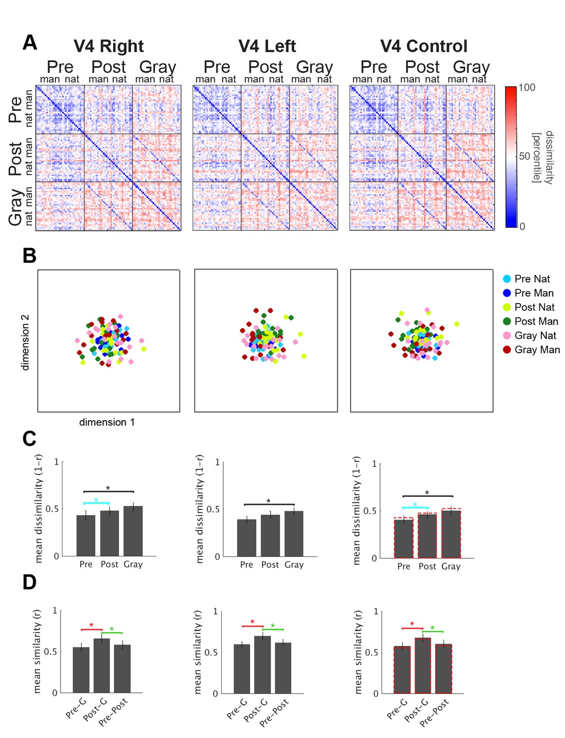
RSA results for the right and left V4 (left and middle column, respectively), and the corresponding ROI size control analysis (right column).
The size of V4 ROIs (right: 256 vx; left: 198 vx) was much smaller than V1-V3 ROIs. Right column: We merged the left and right V4 ROIs for each subject, which yielded ROIs of approximately 500 voxels (mean = 455 vx, s.e.m = 39.1 vx). Again, this analysis yielded very similar results to the original analysis. Red dashed lines in the right column of panels C and D correspond to the original results from right V4 shown in the left column.
Figure 4 with 3 supplements
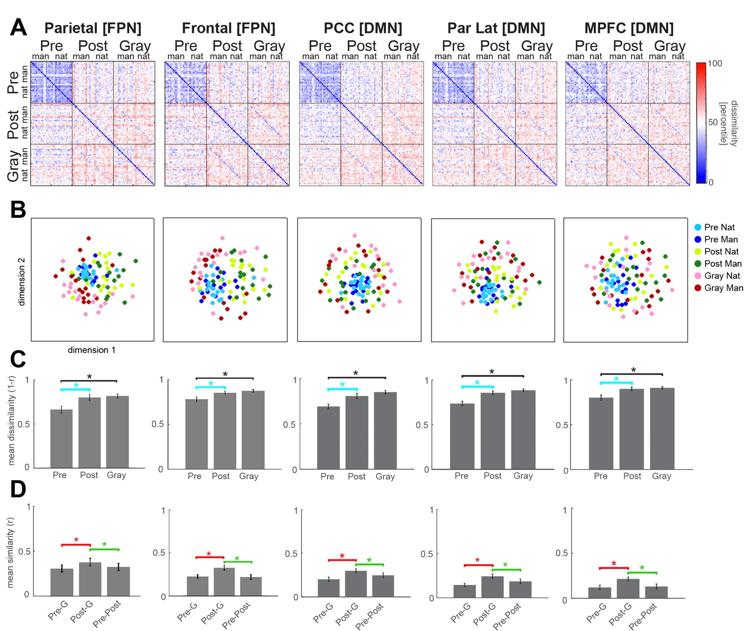
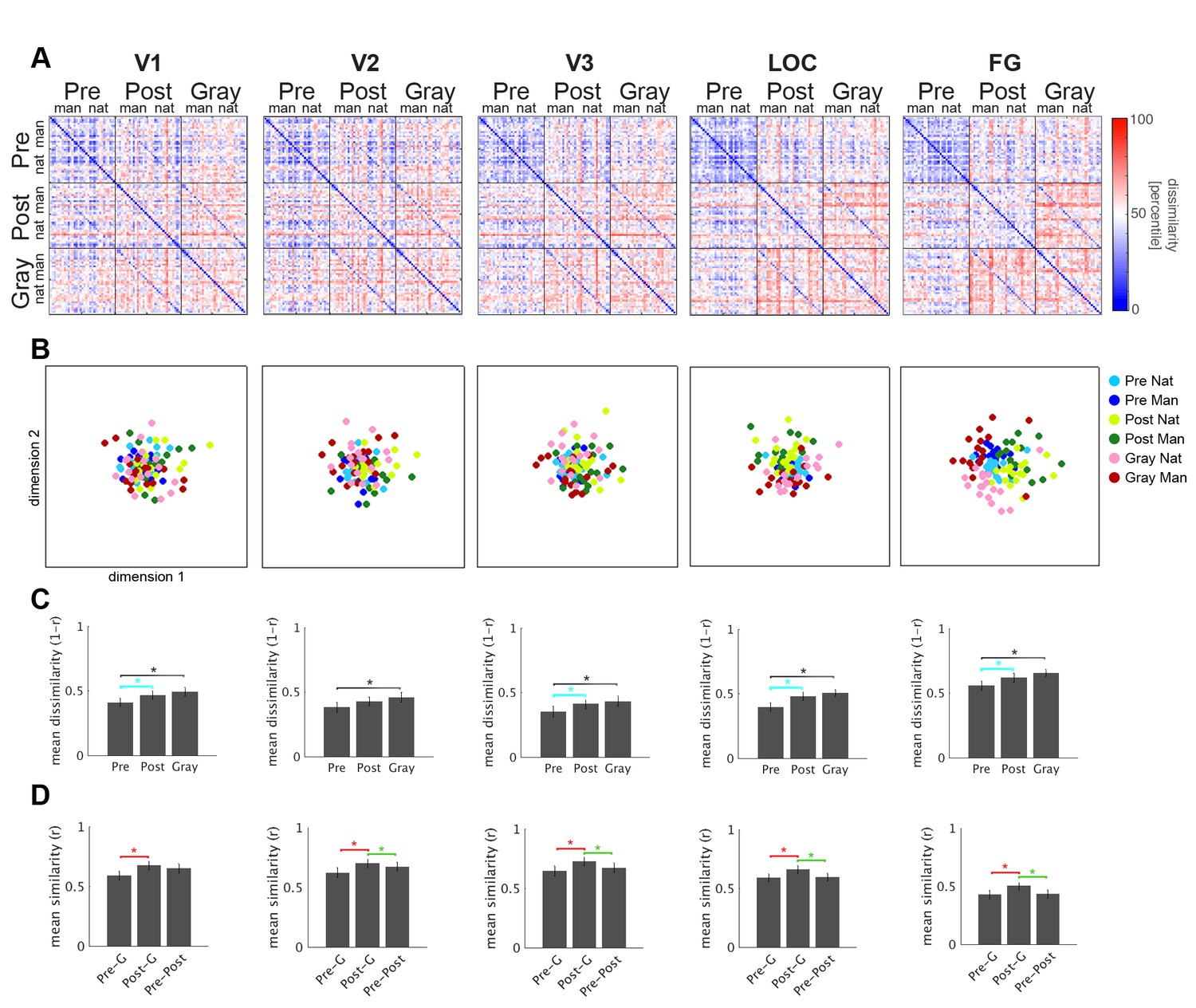
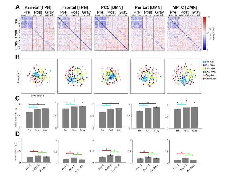
Neural representation format of individual images in frontoparietal regions.
RSA results for FPN and DMN ROIs from the right hemisphere. Format is the same as in Figure 3. Interactive 3-dimensional MDS plots corresponding to first-order RDMs for each ROI can be found at: https://gonzalezgarcia.github.io/mds.html.
Figure 4—figure supplement 1
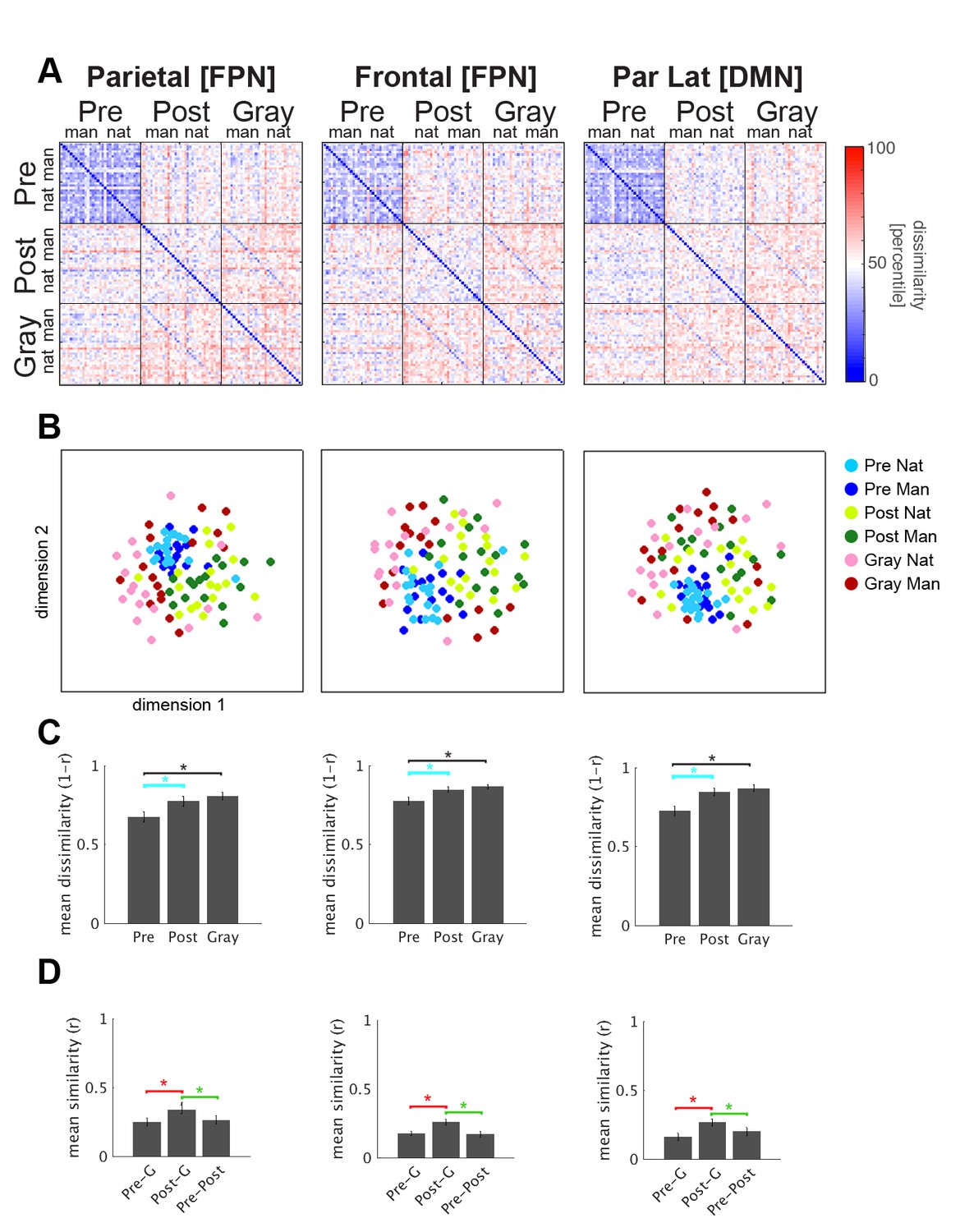
RSA results for left hemisphere FPN and DMN regions.
Same as Figure 4, but for left hemisphere FPN and DMN ROIs, including left parietal and left frontal ROIs from FPN, and left lateral parietal ROI from DMN.
Figure 4—figure supplement 2
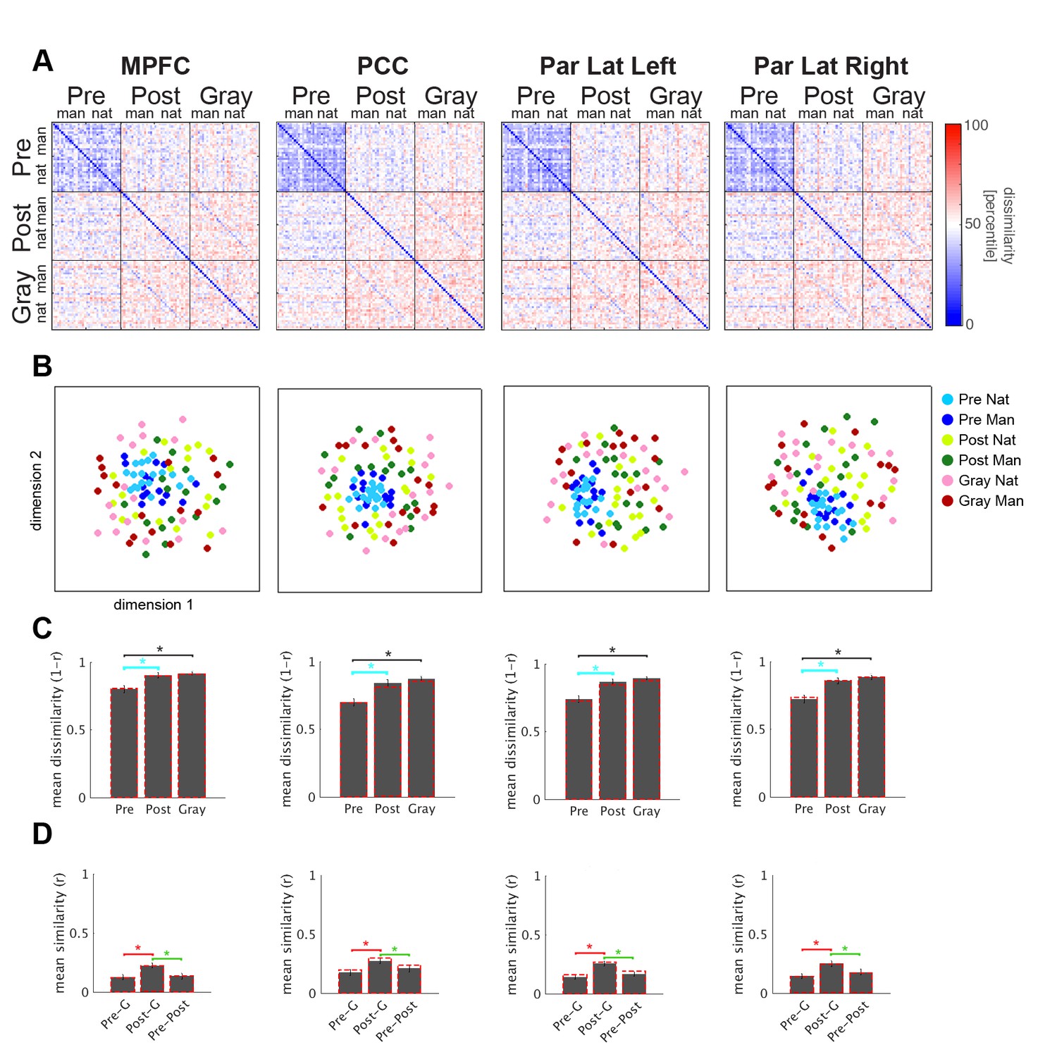
DMN results of the ROI size control analysis.
To assess whether ROI size affected dissimilarity, a control analysis was performed in a subset of regions, including DMN and V4 (V4 results presented in Figure 3—figure supplement 2). We thresholded individual subject’s activation contrast maps (as in Figure 2A) to obtain DMN ROIs of approximately 500 voxels each (mean = 503 vx, s.e.m. = 2.1 vx), which resembled ROI sizes for early visual regions (e.g. 550 voxels for left V1; all ROI sizes are reported in Figure 2—figure supplement 3 legend). Using much smaller DMN ROIs, results very similar to the original analysis (shown here as red dashed line in panels C and D) were found.
Figure 4—figure supplement 3
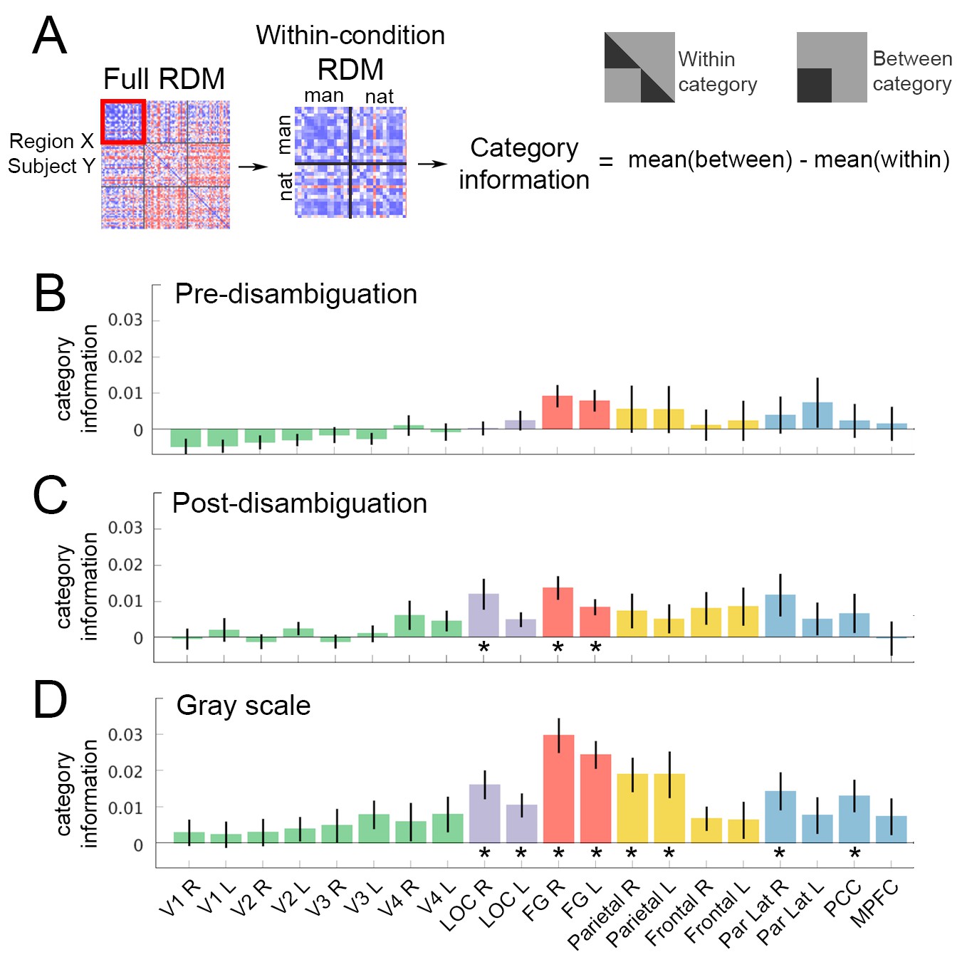
Image category (natural vs.manmade) information.
(A) Analysis schematic. For details, see Materials and methods, RSA. (B–D) Category information in each ROI under each perceptual condition. Bars represent the difference in mean dissimilarity between within-category (Nat-Nat; Man-Man) image pairs and between-category (Nat-Man) image pairs. Error bars denote s.e.m. across subjects. Asterisks denote significantly higher dissimilarity for between-category than within-category elements of the RDM (p<0.05, FDR-corrected, Wilcoxon signed-rank test across subjects).
Figure 5
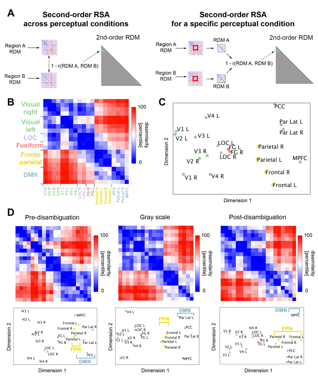
Relationship between neural representation format in different ROIs.
(A) Analysis schematic for second-order RSA across perceptual conditions (left) and within each condition (right). The RDMs from different ROIs were averaged across subjects. Then, a dissimilarity value (1 – Spearman rho) was obtained for each pair of RDMs. (B) Across-condition second-order RDM, depicting the dissimilarities between first-order RDMs of different ROIs. (C) MDS plot corresponding to the second-order RDM show in B. (D) Second-order RDMs and corresponding MDS plots for the pre-disambiguation (left), gray-scale (middle), and post-disambiguation (right) conditions.
-
Figure 5—source data 1
RDM for each ROI in each subject. Includes source code to perform second-order RSA and reproduce Figure 5.
- https://doi.org/10.7554/eLife.36068.017
Figure 6

Dimensionality of neural representation space across ROIs and perceptual conditions.
The dimensionality of neural representation (estimated by the number of dimensions needed in the MDS solution to achieve r2 >0.9) for each ROI, in the pre-disambiguation (A), post-disambiguation (B), and gray-scale (C) condition, respectively. Each bar represents the mean dimensionality averaged across subjects for each ROI. (D) Group-averaged dimensionality for each network and condition. Error bars denote s.e.m. across subjects. Both the network (p=3.1e-16) and the condition (p=2e-6) factors significantly impacted dimensionality, while the interaction was not significant (p=0.29).
-
Figure 6—source data 1
RDM for each ROI in each subject. Includes source code to perform dimensionality analysis and reproduce Figure 6.
- https://doi.org/10.7554/eLife.36068.019
Figure 7
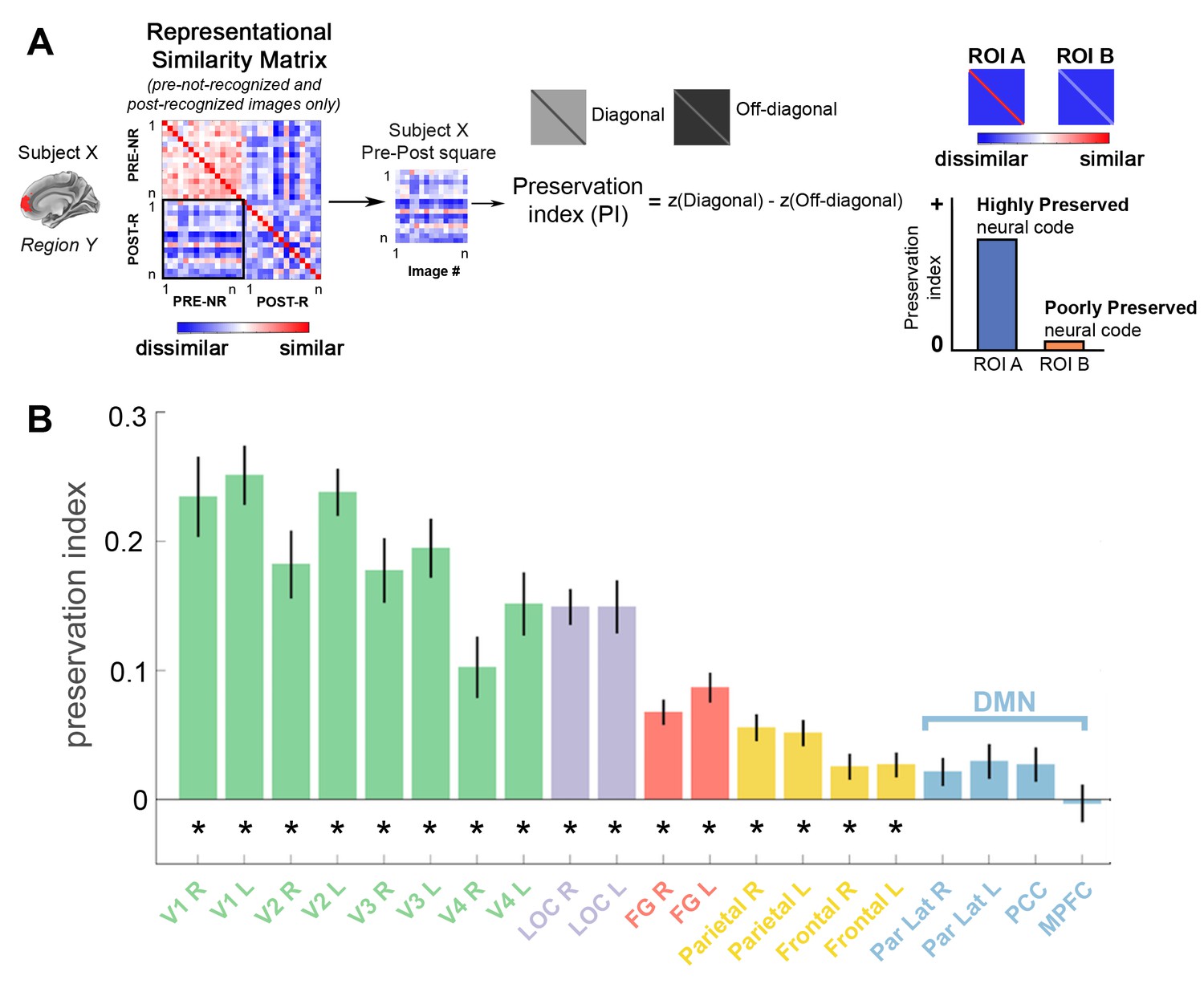
Significant preservation of neural code is found in visual and FPN regions.
(A) Analysis schematic. For each ROI in each subject, a representational similarity matrix (RSM) is constructed using the set of Mooney images that are not recognized in the pre-disambiguation period (PRE-NR) and recognized in the post-disambiguation period (POST-R). The Pre-Post square was extracted from this RSM, and the r-values were Fisher-z-transformed. Then, the difference between diagonal and off-diagonal elements was calculated for each subject, termed ‘Preservation Index’ (PI). A significant positive PI means that a post-disambiguation Mooney image is represented more similarly to the same image than other images shown in the pre-disambiguation period. (B) Group-averaged PI values for each ROI. Error bars denote s.e.m. across subjects. Asterisks denote significant PI values (p<0.05, FDR-corrected, one-sample t-test across subjects).
-
Figure 7—source data 1
RSM (as shown in Figure 7A, left) for each ROI in each subject. Includes source code to perform analysis and reproduce Figure 7.
- https://doi.org/10.7554/eLife.36068.021
Author response image 1
Additional files
-
Transparent reporting form
- https://doi.org/10.7554/eLife.36068.022
Download links
A two-part list of links to download the article, or parts of the article, in various formats.
Downloads (link to download the article as PDF)
Open citations (links to open the citations from this article in various online reference manager services)
Cite this article (links to download the citations from this article in formats compatible with various reference manager tools)
Content-specific activity in frontoparietal and default-mode networks during prior-guided visual perception
eLife 7:e36068.
https://doi.org/10.7554/eLife.36068


