Perceptual processing in the ventral visual stream requires area TE but not rhinal cortex
- National Institute of Mental Health, National Institutes of Health, United States
- National Institute of Advanced Industrial Science and Technology, Japan
- National Institute of Neurological Disorders and Stroke, National Institutes of Health, United States
Figures
Figure 1 with 1 supplement
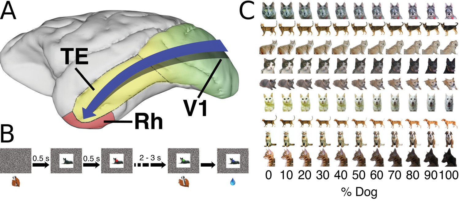
Background and task.
(A) Ventral visual stream - simple features represented in primary visual cortex (green). Increasing complexity of representations in intermediate areas, culminating in the representation of whole objects in area TE (yellow, bounded by dashed line). Immediately rostro-ventral to TE is rhinal cortex (Rh) (red, bounded by solid line - n.b. medial portion of rhinal cortex not visible from this angle). See figure supplement for rhinal cortex reconstructions. (B) A single trial from the perceptual categorization task (see supplemental methods for details). (C) Examples of the cat-dog morphed images presented as visual stimuli in Experiment 1.
Figure 1—figure supplement 1
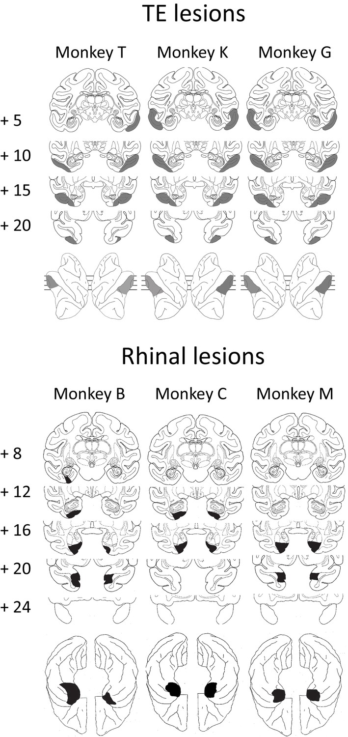
Estimates of the extent of the aspiration lesions of the three monkeys in the TE-lesioned group (top), and rhinal-lesioned group (bottom) are plotted on coronal sections at the indicated levels, and reconstructed onto lateral/ventral views of the macaque brain, respectively; reconstructions for each case are shown at the bottom of each column.
Lesions were reconstructed using MR images (see Matsumoto et al., 2016) for details). Across the groups, lesions largely covered the areas of interest, and damage to adjacent structures was minimal and distributed idiosyncratically across monkeys. TE lesion reconstruction figure modified from Matsumoto et al., 2016, Figure 1; copyright remains with the authors.
Figure 2
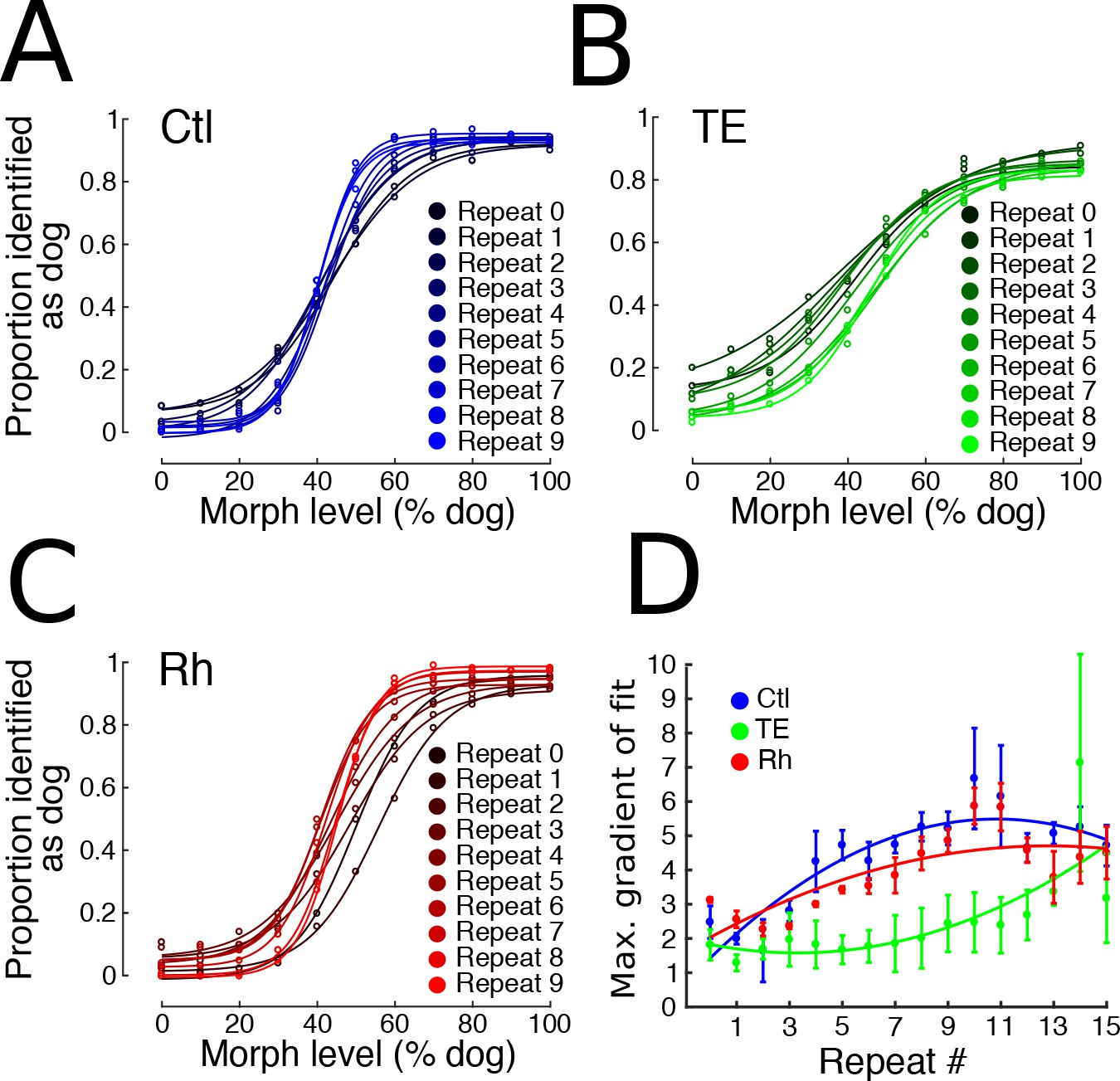
Experiment 1.
(A, B, C) Categorization performance of control (n = 3), TE-lesioned (n = 3), and rhinal-lesioned (n = 3) groups, respectively, during the first 10 presentations of this stimulus set (10 of 16 total presentations plotted for clarity). A steeper gradient to the central portion of the sigmoid indicates higher classification accuracy. Data fit with the function: a + b/(1 + exp(c * x + d)), where a, b, c, and d are free parameters. (D) The maximum slope (±s.e.m.) of the fitted functions in 1C, D and E plotted across presentations, fitted with a quadratic function for each group.
-
Figure 2—source data 1
Experiment 1 - learning to categorize morphed images.
- https://doi.org/10.7554/eLife.36310.005
Figure 3 with 2 supplements
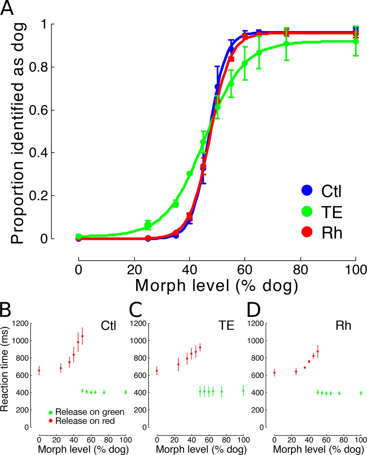
Experiment 2.
(A) Categorization performance of three groups of monkeys: controls (n = 3), TE-lesioned group (n = 3), and Rh-lesioned group (n = 3), mean (±s.e.m.) of presentations 10 to 20. Data fit with the function: a + b/(1 + exp(c * x + d)), where a, b, c, and d are free parameters. (C, D, E) Mean reaction times (±s.e.m.) of control, TE-lesioned, and rhinal-lesioned groups, respectively, for trials ending with a correct response. All trials at the 50% level are included. See figure supplement for stimulus examples.
-
Figure 3—source data 1
Experiment 2 - asymptotic categorization performance.
- https://doi.org/10.7554/eLife.36310.009
Figure 3—figure supplement 1
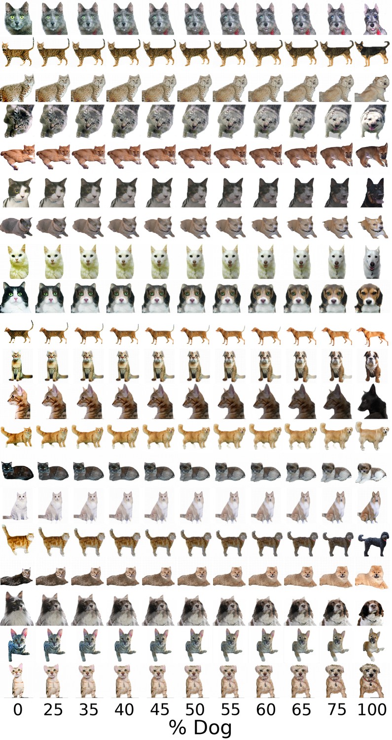
The cat-dog morphed images presented as visual stimuli in Experiment 2.
A total of 20 morph series (one per row) were used for this experiment. Each stimulus was presented once per set, in pseudo-random order; the monkeys completed two sets each day.
Figure 3—figure supplement 2
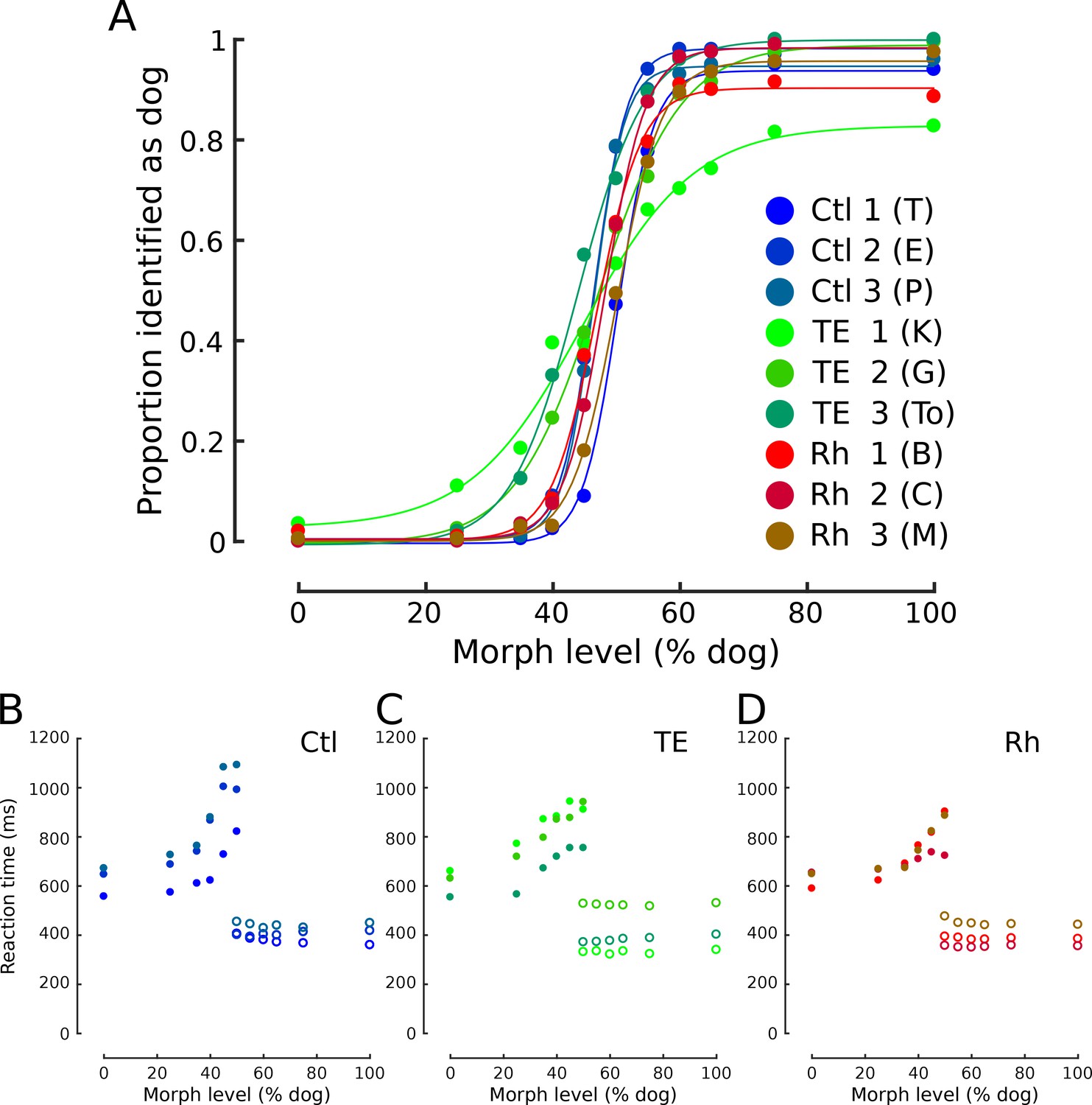
(A) Categorization performance of individual monkeys performing Experiment 2.
Data fit with the function: a + b/(1 + exp(c * x + d)), where a, b, c, and d are free parameters. (C, D, E) Reaction times (±s.e.m.) of individual monkeys for trials ending with a correct response. All trials at the 50% level are included. Monkey-to-color mapping per the legend in ‘A’. Reaction times for bar releases during the presentation of the red target are represented by filled circles, reaction times for releases during the presentation of the green target are represented by open circles.
Figure 4

Visual acuity testing.
Contrast sensitivity is plotted on a logarithmic scale against spatial frequency. Mean sensitivity (±s.e.m.) for each of the three groups of monkeys - controls (n = 3), TE-lesioned group (n = 3), and Rh-lesioned group (n = 3), (six technical replicates per monkey) - is fit with a quadratic function.
-
Figure 4—source data 1
Visual acuity testing.
- https://doi.org/10.7554/eLife.36310.011
Figure 5 with 1 supplement

Experiment 3.
(A) Examples of the visual stimuli presented. Four checker-board masks were placed over each of the stimuli used in Experiment 1, and presented inter-leaved with an unmasked version of each stimulus. (B) Categorization performance of the three test groups: mean (±s.e.m.) of responses to first presentation of all masked stimuli. (C, D, E) Categorization performance on masked (mean of all masks) vs. unmasked stimuli for each group, respectively (first presentation).
-
Figure 5—source data 1
Experiment 3 - categorization of visually degraded stimuli.
- https://doi.org/10.7554/eLife.36310.014
Figure 5—figure supplement 1

(A, C, E) Categorization performance on unmasked stimuli presented in Experiment 3, for individual control (A), TE-lesioned (C), and rhinal-lesioned (E) monkeys.
(B, D, F) Performance on masked (mean of all masks) stimuli (first presentation) for each group: (B) control, (D) TE-lesioned, (F) rhinal-lesioned.
Figure 6 with 2 supplements
Experiment 4.
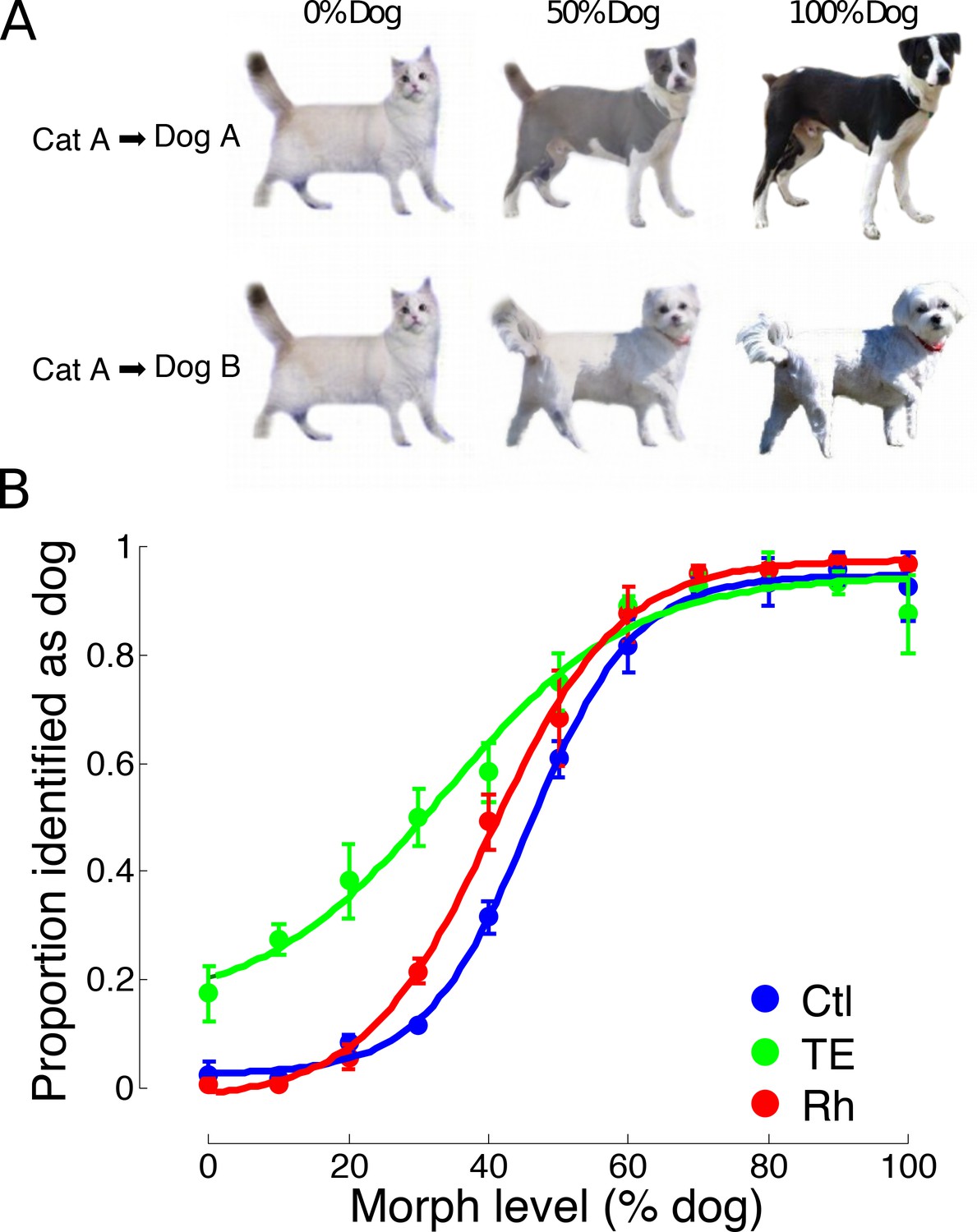
(A) Examples of the visual stimuli presented; each cat was morphed with two dogs, and vice versa, for example Cat A was morphed with Dog A (top row), and with Dog B (bottom row). Examples at the 0%, 50%, and 100% dog level are shown; the full set of stimuli used in Experiment 4 was distributed across the same morph levels as used in Experiment 1 (see figure supplement for a larger set of stimulus examples). (B) Mean categorization performance (±s.e.m.) of the three test groups with a single presentation of each stimulus.
-
Figure 6—source data 1
Experiment 4 - categorization of novel stimuli.
- https://doi.org/10.7554/eLife.36310.018
Figure 6—figure supplement 1

Examples of the cat-dog morphed images presented as visual stimuli in Experiment 4.
Twelve morph series – one on each row – are shown. A total of 40 morph series were used for this experiment. Each stimulus was presented once, in pseudo-random order; the monkeys completed a single session.
Figure 6—figure supplement 2

Categorization performance of individual monkeys in Experiment 4, in which each stimulus was novel, and presented only once.
https://doi.org/10.7554/eLife.36310.017Additional files
-
Transparent reporting form
- https://doi.org/10.7554/eLife.36310.019
Download links
A two-part list of links to download the article, or parts of the article, in various formats.
Downloads (link to download the article as PDF)
Open citations (links to open the citations from this article in various online reference manager services)
Cite this article (links to download the citations from this article in formats compatible with various reference manager tools)
Perceptual processing in the ventral visual stream requires area TE but not rhinal cortex
eLife 7:e36310.
https://doi.org/10.7554/eLife.36310


