Quantification of gene expression patterns to reveal the origins of abnormal morphogenesis
- The Barcelona Institute for Science and Technology, Spain
- Universitat Pompeu Fabra, Spain
- European Molecular Biology Laboratory, Spain
- Universitat de Barcelona, Spain
- Universitat de les Illes Balears (UIB), Spain
- Pennsylvania State University, United States
- Institució Catalana de Recerca i Estudis Avançats, Spain
Figures
Figure 1
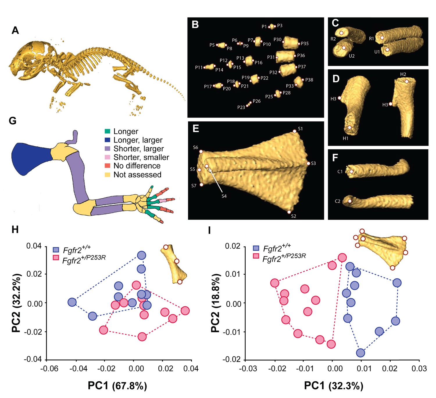
Quantitative size and shape comparison of forelimb bones in Fgfr2+/P253R newborn mice (P0) and unaffected littermates.
(A) Mouse skeleton at P0. 3D isosurface reconstruction of the skeleton of an unaffected littermate obtained from a high-resolution µCT scan. (B–F) Anatomical landmarks recorded on microCT scans of Apert syndrome mice at P0. (B) Autopod (hand). Landmarks were recorded at the midpoint of the proximal and distal tips of the distal, mid and proximal phalanges (P1–P28) and the metacarpals (P29–P38). Proximal phalanx I, middle phalanx V, and metacarpal I are not displayed because these bones have not yet mineralized at P0 and could not be visualized in many specimens. (C) Zeugopod. Landmarks were recorded at the midpoint of the proximal and distal tips of the radius (R1–R2) and ulna (U1–U2). (D) Stylopod. Landmarks were recorded at the midpoint of the proximal and distal tips of the humerus (H1–H2), as well as at the tip of the deltoid process (H3) (Figure 1—source data 1). (E) Scapula. Landmarks were recorded at the most superior and inferior lateral points of the scapula (S1–S2), the most posterior point of the spine (S3), the most antero-medial point of the acromion process (S4) and the medial, superior and inferior points of the glenoid cavity (S5–S7) (Figure 1—source data 2). (F) Clavicle. Landmarks were recorded at the medial point of the sternal and the acromial ends (C1–C2). (G) Length and volume differences in the forelimbs of Apert syndrome mouse models. Schematic representation of the forelimb of a P0 mouse showing, in different colors, statistically significant differences in bone length and volume (as measured by two-tailed one-way ANOVA or Mann-Whitney U-test) in Fgfr2+/P253R mice and unaffected littermates, as specified in Table 1. Longer/shorter refers to length, whereas larger/smaller refers to volume. (H, I) Shape differences in the forelimbs of Apert syndrome mouse models. Scatterplots of PC1 and PC2 scores based on Procrustes analysis of anatomical landmark locations representing the shape of the left humerus (H) and the left scapula (I) of unaffected (N = 10) and mutant (N = 12) littermates of Apert syndrome mouse models (Figure 1—source data 1 and Figure 1—source data 2). Convex hulls represent the range of variation within each group of mice.
-
Figure 1—source data 1
Source files for humerus shape data.
This zip archive contains the i) raw landmark coordinates registered to capture the shape of the humerus, as defined in Figure 1D; ii) the estimated centroid size and long-centroid size; iii) the Procrustes coordinates after Generalized Procrustes analysis (GPA); and iv) the PC scores resulting from the Principal Component Analysis (PCA) displayed in Figure 1H.
- https://doi.org/10.7554/eLife.36405.004
-
Figure 1—source data 2
Source files for scapula shape data.
This zip archive contains the (i) raw landmark coordinates registered to capture the shape of the scapula, as defined in Figure 1E; (ii) the estimated centroid size and long-centroid size; iii) the Procrustes coordinates after Generalized Procrustes Analysis (GPA); and iv) the PC scores resulting from the Principal Component Analysis (PCA) displayed in Figure 1I.
- https://doi.org/10.7554/eLife.36405.005
Figure 2
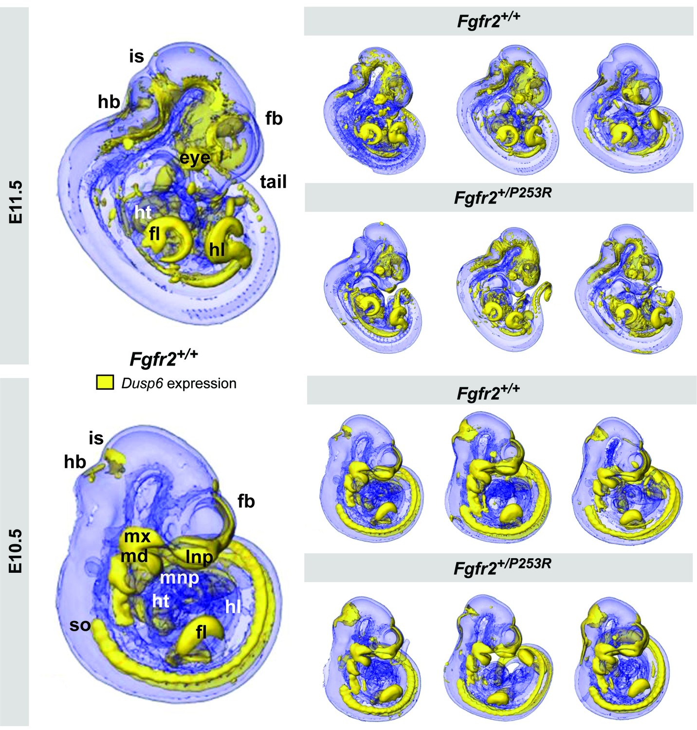
Qualitative visualization of Dusp6 gene expression in unaffected and Fgfr2+/P253R mouse embryos at E10.5 and E11.5.
OPT scans of embryos WMISH stained for Dusp6 revealed the anatomical location of Dusp6 gene expression (shown in yellow). For each stage, the main expression domains are highlighted on the left for anatomical reference on a lateral view of a 3D reconstruction of a Fgfr2+/+ unaffected embryo (fb, forebrain; fl, forelimb; hb, hindbrain; hl, hindlimb; ht, heart; is, isthmus; lnp, lateral nasal process; md, mandibular prominence; mnp, medial nasal process; mx, maxillary prominence; so, somites). On the right, 3D reconstructions of three unaffected and three Fgfr2+/P253R mutant embryos from the same litter are displayed to represent the high degree of variation in developmental age within litters. Embryos are not to scale. Original 2D images of the Dusp6 WMISH experiments are available in Figure 2—source data 1.
-
Figure 2—source data 1
Original 2D images of the Dusp6 WMISH experiments.
This zip archive contains pictures, taken using a Leica MX16F microscope, of the right and left sides of the mouse embryos that underwent Dusp6 WMISH. Folders are organized by developmental stage and genotype.
- https://doi.org/10.7554/eLife.36405.008
Figure 3
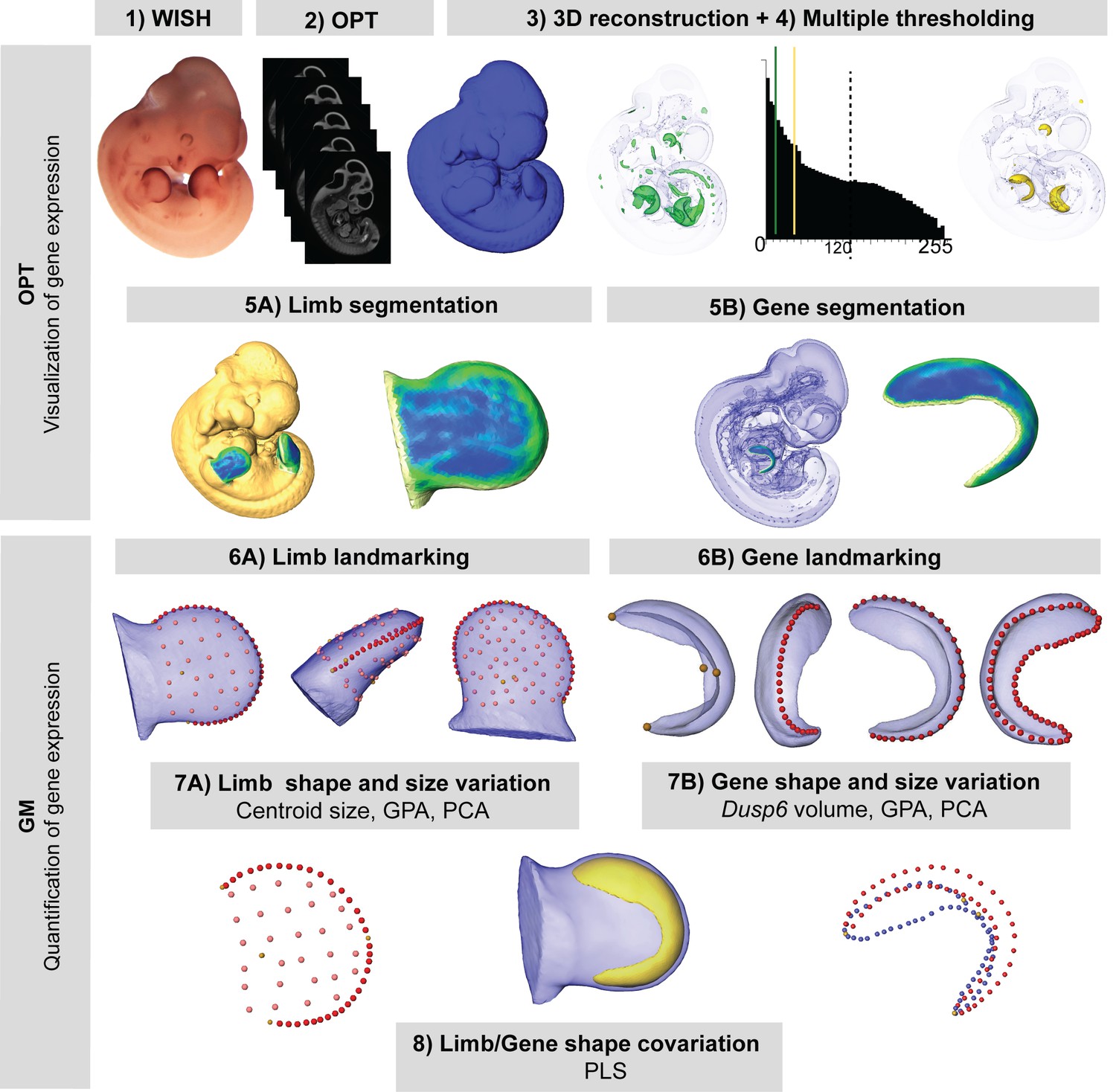
New quantitative analysis method for 3D gene expression data, based on Geometric Morphometrics.
Mouse embryos between E10.5 and E11.5 were analyzed with WMISH to reveal the expression of Dusp6 (1), and then cleared with BABB, and OPT scanned using both fluorescence and transmission light (2). The external surface of the embryo was obtained from the 3D reconstruction of the fluorescence scan (2). Multiple thresholding of the transmission scan by choosing different levels of grey values as shown by the histogram allowed the visualization of gene expression patterns at different intensities (3). Moderate gene expression (shown in green) was displayed as the isosurface obtained using a threshold of the grey value computed as 2/3 of the last grey value showing the Dusp6 expression domain (3). High gene expression (shown in yellow) was displayed as the isosurface obtained using a threshold of the grey value computed as 1/3 of the last grey value showing the Dusp6 expression domain (3). From the whole mouse embryo isosurfaces, all four limb buds were segmented (5A). From the high gene expression isosurface, the Dusp6 domains from all of the available limbs were segmented (5B). Maximum curvature patterns were displayed to optimize landmark recording (5). For each limb, we captured the shape and size of the limb bud (6A) and the underlying high Dusp6 gene expression pattern (6B), recording the 3D coordinates of anatomical landmarks (yellow dots), curve semi-landmarks (red dots) and surface semi-landmarks (pink dots). Anatomical and curve landmarks were recorded manually on each limb. Surface landmarks were recorded on one template limb and interpolated onto target limbs (Video 1). Landmark coordinates were the input for Geometric Morphometric (GM) quantitative shape analysis (7, 8) that was used to superimpose the landmark data (GPA, Generalized Procrustes Analysis), to compute limb size (centroid size), and to explore both shape variation within limbs and gene expression domains within litters by Principal Component Analysis (PCA). Finally, the covariation patterns for the shape of the limb and the shape of the gene expression domain were also explored using the Partial Least Squares (PLS) method.
Figure 4

Developmental variation within litters of the Apert syndrome mouse model.
All of the limbs were individually staged using our publicly available web-based staging system (https://limbstaging.embl.es). The stage of the limb bud was estimated after alignment and shape comparison of the spline with an existing dataset with a reproducibility of ±2 hr. As both Litter 1 and Litter 2 comprised limbs between E10 and E10.5, we pooled these limbs into the 'Early' period. Litter 3, comprising limbs between E10 and E11, represented the 'Mid' developmental period. And finally, Litter 4, which included limbs between E11 and E11.5, was considered as the 'Late' period. In subsequent analyses, forelimbs and hindlimbs were analyzed separately, as specified in Table 2. Increasing color intensities in dots represent an increasing number of limbs with the same staging result. Individual scores are available in Figure 4—source data 1.
-
Figure 4—source data 1
Staging results.
Table containing the individual scores obtained from the staging system and used to produce the graph in Figure 4.
- https://doi.org/10.7554/eLife.36405.012
Figure 5 with 3 supplements
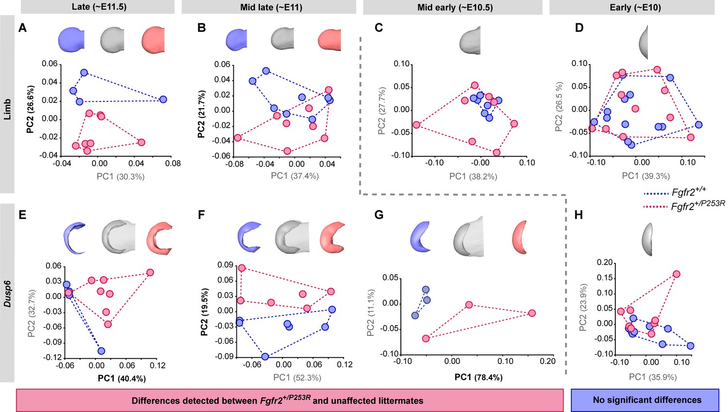
Tracing of limb phenotypes (anatomical and molecular) back through developmental time to the earliest moment of appearance.
Principal Component Analysis based on the Procrustes-based semi-landmark analysis was used to assess the shape of the limbs and the corresponding Dusp6 expression domains for each developmental period (Figure 5—figure supplement 1). Each period was analyzed separately for the shape of the limb (A–D) and the Dusp6 expression domain (E–H), as specified in the 'Materials and methods' and in Table 2. Scatterplots of PC1 and PC2 axes with the corresponding percentages of total morphological variation explained are displayed for each analysis, along with the morphings associated with the negative, mid and positive values of the PC axis that separates mutant and unaffected littermates (PC1 or PC2, as highlighted in bold black letters in the corresponding axis). Morphings are displayed in grey tones when the analysis showed no differentiation between mutant and unaffected littermates. Morphings are displayed in color when the analysis revealed differentiation between mouse groups (blue: unaffected littermates; pink: mutant littermates). Limb buds and Dusp6 domains are not to scale and are oriented with the distal aspect to the left, the proximal aspect to the right, the anterior aspect at the top and the posterior aspect at the bottom of all images. Convex hulls represent the ranges of variation within each group of mice. Individual scores are available in Figure 5—source data 1. Results from the complete dataset analyzing hindlimbs (Figure 5—figure supplement 2, Figure 5—figure supplement 2—source data 1) and forelimbs (Figure 5—figure supplement 3, Figure 5—figure supplement 3—source data 1) from each litter separately are also available.
-
Figure 5—source data 1
Source files for limb shape data.
This zip archive contains the (i) raw landmark coordinates registered to capture the shape of the limbs and the associated Dusp6 expression domains, as defined in Figure 5—figure supplement 1; (ii) the estimated centroid size and long-centroid size of each structure; (iii) the Procrustes coordinates after Generalized Procrustes Analysis (GPA); and iv) the PC scores resulting from each of the Principal Component Analyses (PCA) displayed in Figure 5.
- https://doi.org/10.7554/eLife.36405.020
Figure 5—figure supplement 1
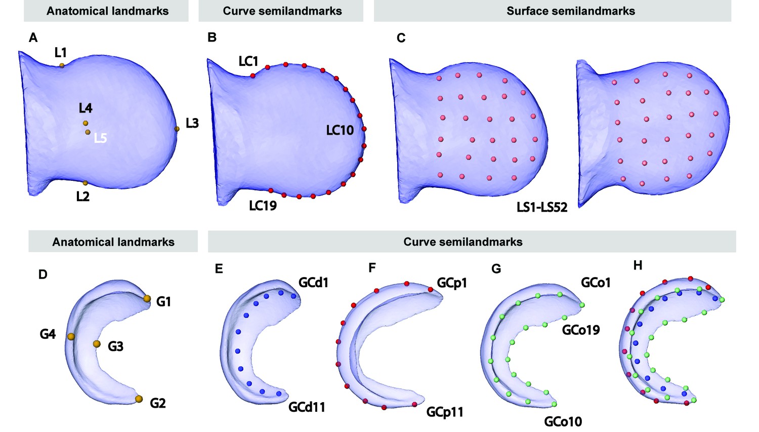
Anatomical landmarks recorded on the 3D reconstructions of the limbs and the Dusp6 expression domains obtained from OPT scans of Apert syndrome embryos at E10.5–E11.5.
In the limb, we manually recorded the 3D coordinates of five anatomical landmarks (A): L1–L2, the most medial points on the anterior and the posterior sides of wrist, collected along the curve that divides the limb on the dorsal and ventral sides; L3, the most distal point of the limb, collected along the curve that divides the limb on the dorsal and ventral sides; and L4–L5, the most superior and inferior points on the dorsal and ventral sides of the limb. We also recorded between 25 and 60 points along the curve that divides the limb on the dorsal and ventral sides to define an outline spline of the limb. Using Viewbox 4, we obtained the 3D coordinates of 19 equidistant points along the outline spline that were considered in further comparative shape analyses to be curve semi-landmarks (LC1–LC19) (B). Finally, we recorded 52 surface semi-landmarks on the dorsal and ventral sides of the limb interpolating the points from a reference limb to each target limb, using the five anatomical landmarks manually recorded as matching points and by minimizing the bending energy (LS1–LS52) (C). In the gene, we manually recorded the 3D coordinates of four anatomical landmarks (D): G1–G2, the points at the most anterior and posterior tips of the gene expression domain; G3-G4, the points at the maximum curvature of the proximal side of the gene expression domain, on the dorsal and the ventral sides (D). (We also recorded 10–30 points along the distal and proximal curves of the gene expression domain at the sagittal plane, and 30–60 points along the outline of the gene expression domain, on its proximal side.) Using Viewbox 4, we obtained the 3D coordinates of eleven equidistant points along the spline of the distal and proximal curves of the gene expression domain (GCd1–GCd11 and GCp1–GCp11) (E and F), and 19 equidistant points along outline of the gene expression domain, on its proximal side (GCo1–GCo19) (G) that were considered in further comparative shape analyses as curve semi-landmarks, and are displayed simultaneously in (H).
Figure 5—figure supplement 2
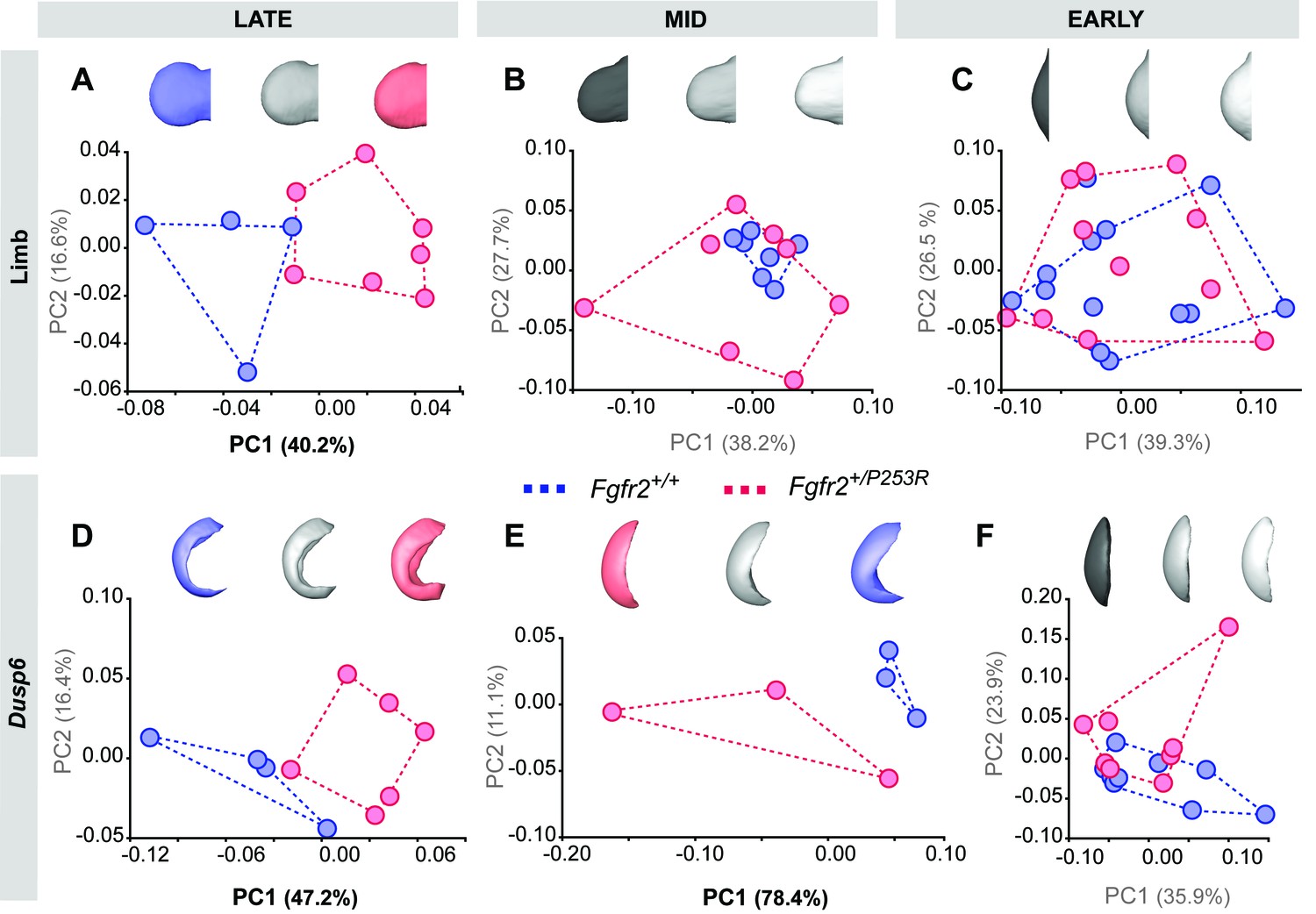
Principal Component analyses based on the Procrustes-based semi-landmark analysis of the shape of the hindlimbs and the corresponding Dusp6 expression domains for each developmental period.
Scatterplots of PC1 and PC2 axes with the corresponding percentage of total morphological variation explained are displayed for each analysis, along with morphings associated with the negative, mid and positive values of the PC axis that separates mutant and unaffected littermates (PC1 or PC2, as highlighted in bold black letters in the corresponding axis). Morphings are displayed in grey tones when the analysis shows no differentiation between unaffected and mutant littermates. Morphings are displayed in color when the analysis reveals differentiation between the mouse groups (blue: unaffected littermates; pink: mutant littermates). Limb buds and Dusp6 domains are not to scale and are oriented distally to the left, proximally to the right, anteriorly to the top and posteriorly to the bottom. Convex hulls represent the ranges of variation within each group of mice, as defined in Table 2 and Figure 4. Individual scores are available in Figure 5—figure supplement 2—source data 1.
-
Figure 5—figure supplement 2—source data 1
Source files for hindlimb shape data.
This zip archive contains the i) raw landmark coordinates registered to capture the shape of the hindlimbs and the associated Dusp6 expression domains, as defined in Figure 5—figure supplement 1; ii) the estimated centroid size and long-centroid size of each structure; iii) the Procrustes coordinates after Generalized Procrustes Analysis (GPA); and iv) the PC scores resulting from each of the Principal Component Analyses (PCA) displayed in Figure 5—figure supplement 2.
- https://doi.org/10.7554/eLife.36405.017
Figure 5—figure supplement 3
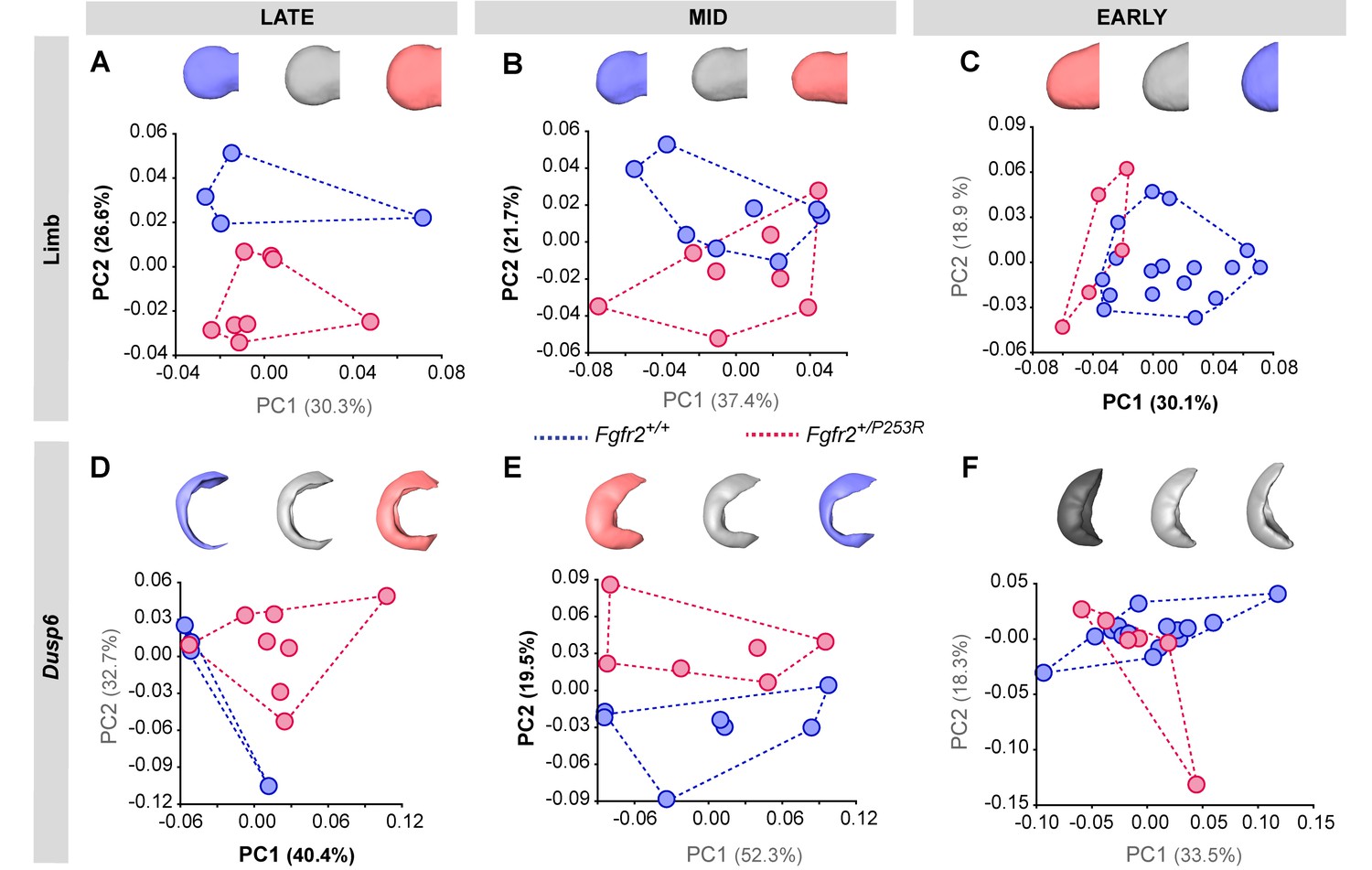
Principal Component analyses based on the Procrustes-based semi-landmark analysis of the shape of the forelimbs and the corresponding Dusp6 expression domains for each developmental period.
Scatterplots of PC1 and PC2 axes with the corresponding percentage of total morphological variation explained are displayed for each analysis, along with morphings associated with the negative, mid and positive values of the PC axis that separates mutant and unaffected littermates (PC1 or PC2, as highlighted in bold black letters in the corresponding axis). Morphings are displayed in grey tones when the analysis shows no differentiation between unaffected and mutant littermates. Morphings are displayed in color when the analysis reveals differentiation between the mouse groups (blue: unaffected littermates; pink: mutant littermates). Limb buds and Dusp6 domains are not to scale and are oriented distally to the left, proximally to the right, anteriorly to the top and posteriorly to the bottom. Convex hulls represent the ranges of variation within each group of mice, as defined in Table 2 and Figure 4. Individual scores are available in Figure 5—figure supplement 3—source data 1.
-
Figure 5—figure supplement 3—source data 1
Source files for forelimb shape data.
This zip archive contains the i) raw landmark coordinates registered to capture the shape of the forelimbs and the associates Dusp6 expression domains, as defined in Figure 5—figure supplement 1; ii) the estimated centroid size and long-centroid size of each structure; iii) the Procrustes coordinates after Generalized Procrustes Analysis (GPA); and iv) the PC scores resulting from each of the Principal Component Analyses (PCA) displayed in Figure 5—figure supplement 3.
- https://doi.org/10.7554/eLife.36405.019
Figure 6 with 2 supplements
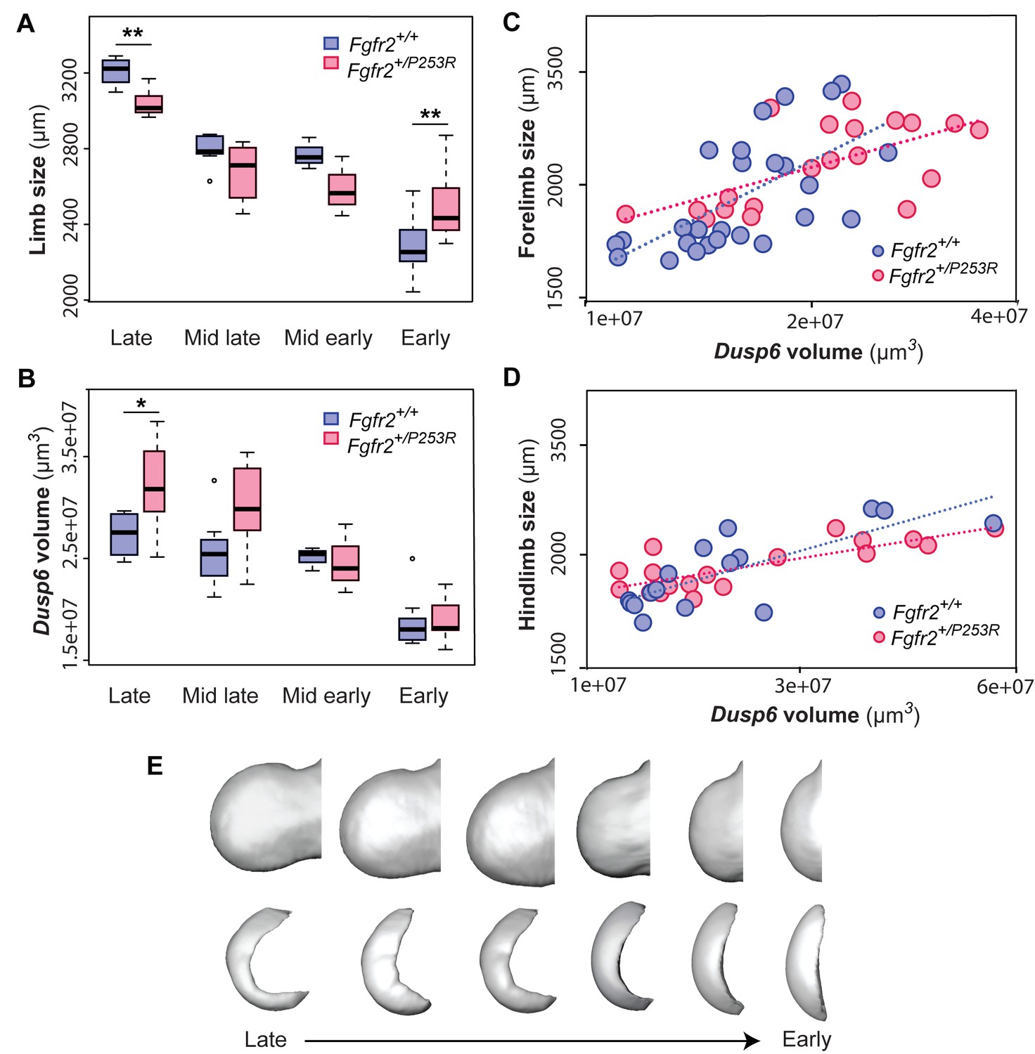
Quantitative correlation between the size and shape of the limbs and the Dusp6 expression pattern.
(A–D) Comparison of limb bud size and Dusp6 volume in unaffected and Fgfr2+/P253R mutant littermates across development (Table 3). Limb size was measured as limb centroid size (A), whereas the size of the Dusp6 expression was measured as the volume of the gene domain (B), as specified in the 'Materials and methods' and in Table 2. Statistically significant differences as revealed by two-tailed t-tests are marked with asterisks, representing the degree of significance: *P-value=0.03, **P-value=0.01. Results from hindlimbs and forelimbs are separately available in Figure 6—figure supplement 1. The association between the size of the limbs and the volume of the Dusp6 domain was assessed separately for forelimbs (C) and hindlimbs (D). Individual scores for all of these analyses are available in Figure 6—source data 1. (E) Time course assessing the morphological integration pattern between the limb phenotype and the shape of the gene expression pattern using partial least squares analyses. Associated shape changes from late to early limb development are shown from morphings associated with the negative, mid and positive values of PLS1, which accounted for almost all of the covariation (97.6% in forelimbs and 99.5% in hindlimbs) between the limb buds and the Dusp6 gene expression domains (Figure 6—figure supplement 2). Limb buds and Dusp6 domains are not shown to scale and are oriented distally to the left, proximally to the right, anteriorly to the top and posteriorly to the bottom. On the right, representing the positive extreme of PLS1 axis, typical early limb buds showed a protruding shape (i.e. short in the proximo-distal axis and symmetrical in the antero-posterior axis) associated with a flat-bean shaped Dusp6 expression zone localized in the distal limb region, underlying the apical ectodermal ridge and spreading proximally towards the dorsal and ventral sides of the limb. On the left, representing the negative extreme of the PLS1 axis, limb buds were elongated in the proximal axis and asymmetric on the antero-posterior axis, with an expansion of the distal limb region and a contraction of the proximal region, at the wrist level. This limb shape, which is typical of more developed limbs, was associated with a Dusp6 expression that was extended underneath the apical ectodermal ridge towards the anterior and the posterior ends of the gene expression zone, but reduced on the dorsal and ventral sides of the limb. Individual scores for all of these analyses are available in Figure 6—figure supplement 2—source data 1. Legends for supplementary figures.
-
Figure 6—source data 1
Source files for limb size and gene expression volume.
This Excel file contains tables with the individual scores for limb centroid size (µm) and Dusp6 volume (µm3) used to produce the graphs in (i) Figure 6A and Figure 6B; (ii) Figure 6C and Figure 6—figure supplement 1B,D; and (iii) Figure 6D and Figure 6—figure supplement 1A,C.
- https://doi.org/10.7554/eLife.36405.025
Figure 6—figure supplement 1
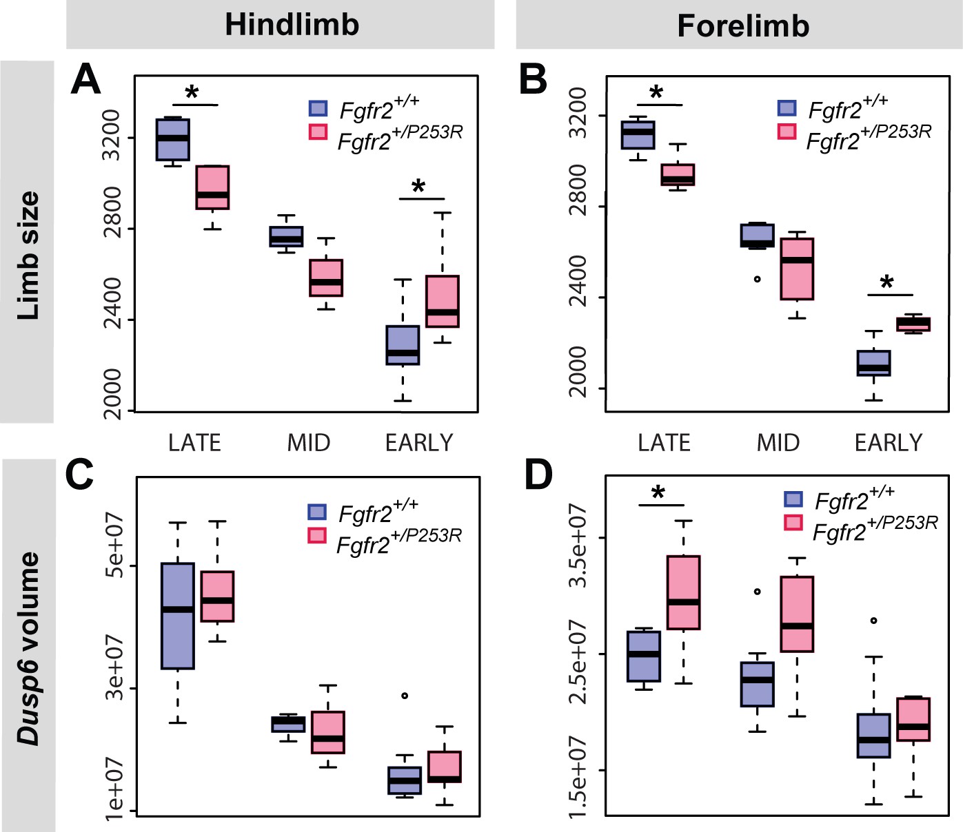
Quantitative size analyses of limb bud and Dusp6 volume in unaffected and Fgfr2+/P253R mutant littermates throughout development.
Comparison in hindlimbs (A, C) and forelimbs (B, D) at each developmental period, as defined in Table 2 and Figure 4. Limb size was measured in terms of limb centroid size (μm), whereas the size of the Dusp6 expression zone was measured as the volume of the gene expression domain (μm3). Statistical significant differences as revealed by two-tailed t-tests are marked with asterisks: *P-value<0.05. Individual scores are available in Figure 6—source data 1.
Figure 6—figure supplement 2

Morphological integration between the shapes of the limb bud and the Dusp6 gene expression domain, as measured by partial least square (PLS) analysis.
Results display the morphings associated with the negative, mid and positive values of PLS1 for hindlimbs (A) and forelimbs (B), which accounted for more than 95% of the covariation between the limb buds and the Dusp6 gene expression domains. Separate PLS analyses for hindlimbs (C) and forelimbs (D) for each developmental group, as defined in Table 2 and Figure 4, are also shown. Formal testing of differences in the intensity of the integration patterns in unaffected and Fgfr2+/P253R mutant mice at each stage was not possible because of sample size limitations, as specified in 'Materials and methods' and in Table 2. Individual scores are available in Figure 6—figure supplement 2—source data 1. Rich media.
-
Figure 6—figure supplement 2—source data 1
Results of Ppartial Least Squares (PLS) analyses.
This zip archive contains the PLS scores resulting from each of the analyses displayed in Figure 6—figure supplement 2.
- https://doi.org/10.7554/eLife.36405.024
Videos
Video 1
Morphometric approach for the analysis of 3D gene expression data obtained by Optical Projection Tomography.
In this video, we show a superimposed view of a fluorescent and a transmission OPT scan of the same E11.5 mouse embryo, which was analyzed with WMISH to reveal the gene expression of Dusp6, a downstream target of Fgf signaling. The surface of the mouse embryo rotating around its central axis was obtained from the 3D reconstruction of an OPT scan based on fluorescence light. The expression pattern of the Dusp6 gene was segmented from the transmission OPT scan using multiple thresholding. The imaging revealed the anatomical location of regions of high Dusp6 gene expression (shown in purple). To compare unaffected and Fgfr2+/P253R mouse embryos and to detect statistically significant differences between them, we collected landmarks along the surface of the gene expression domain (yellow dots) and the limb bud (green dots), which capture the size and shape of the limb and the underlying gene expression domain to a highly accurate level of detail. Further quantitative analyses provided insight into the origins of limb malformations in Apert syndrome.
Tables
Table 1
Quantitative comparison of mean bone lengths and volumes.
Means were computed as the average lengths or volumes of the right and the left bones for Fgfr2+/P253R mutant (N = 12) and Fgfr2+/+ unaffected (N = 10) mice. Data for proximal phalanx I, middle phalanx V, and metacarpal I are not listed because these bones were not present in all of the specimens, as they may not yet be developed at P0. Statistically significant differences as determined by two-tailed one-way ANOVA or Mann-Whitney U-tests are marked with * (P-value<0.05). Statistically significant differences after Bonferroni correction are indicated with **.
| Mean bone length (mm ± SD) | Mean bone volume (mm3 ± SD) | ||||||
|---|---|---|---|---|---|---|---|
| Bone | Fgfr2+/+ | Fgfr2+/P253R | P-value | Fgfr2+/+ | Fgfr2+/P253R | P-value | |
| Autopod | Distal phalanx I | 0.11 ± 0.03 | 0.13 ± 0.02 | 0.004** | 0.0015 ± 0.0008 | 0.0015 ± 0.0008 | 0.86 |
| Distal phalanx II | 0.22 ± 0.03 | 0.21 ± 0.03 | 0.128 | 0.0021 ± 0.0007 | 0.0022 ± 0.0008 | 0.659 | |
| Middle phalanx II | 0.004 ± 0.003 | 0.01 ± 0.004 | 0.336 | 0.00002 ± 0.00002 | 0.00003 ± 0.00002 | 0.759 | |
| Proximal phalanx II | 0.15 ± 0.01 | 0.14 ± 0.01 | 0.057 | 0.0054 ± 0.0011 | 0.0053 ± 0.0014 | 0.82 | |
| Distal phalanx III | 0.26 ± 0.006 | 0.24 ± 0.01 | 0.068 | 0.0034 ± 0.0008 | 0.0033 ± 0.0017 | 0.796 | |
| Middle phalanx III | 0.10 ± 0.006 | 0.10 ± 0.006 | 0.243 | 0.0019 ± 0.0009 | 0.0022 ± 0.0013 | 0.436 | |
| Proximal phalanx III | 0.204 ± 0.02 | 0.18 ± 0.03 | 0.001** | 0.0087 ± 0.0003 | 0.0073 ± 0.0004 | 0.016* | |
| Distal phalanx IV | 0.24 ± 0.006 | 0.19 ± 0.02 | 0.061 | 0.0024 ± 0.0009 | 0.0024 ± 0.0014 | 0.923 | |
| Middle phalanx IV | 0.06 ± 0.009 | 0.07 ± 0.01 | 0.338 | 0.0009 ± 0.0002 | 0.0014 ± 0.0002 | 0.24 | |
| Proximal phalanx IV | 0.20 ± 0.01 | 0.20 ± 0.02 | 0.412 | 0.0080 ± 0.0016 | 0.0075 ± 0.0021 | 0.358 | |
| Distal phalanx V | 0.09 ± 0.01 | 0.08 ± 0.01 | 0.832 | 0.0005 ± 0.00007 | 0.0006 ± 0.0001 | 0.769 | |
| Proximal phalanx V | 0.14 ± 0.01 | 0.15 ± 0.02 | 0.027* | 0.0031 ± 0.0007 | 0.0036 ± 0.0012 | 0.089 | |
| Metacarpal II | 0.39 ± 0.02 | 0.41 ± 0.02 | 0.034* | 0.0270 ± 0.0028 | 0.0265 ± 0.0034 | 0.586 | |
| Metacarpal III | 0.49 ± 0.03 | 0.52 ± 0.03 | 0.004* | 0.0398 ± 0.0043 | 0.0382 ± 0.0062 | 0.342 | |
| Metacarpal IV | 0.43 ± 0.02 | 0.45 ± 0.03 | 0.011* | 0.0312 ± 0.0033 | 0.0291 ± 0.0048 | 0.114 | |
| Metacarpal V | 0.22 ± 0.01 | 0.22 ± 0.02 | 0.571 | 0.0120 ± 0.0019 | 0.0124 ± 0.0023 | 0.458 | |
| Zeugopod | Radius | 2.29 ± 0.02 | 2.22 ± 0.01 | 0.003* | 0.3187 ± 0.0292 | 0.3558 ± 0.0334 | 0.001** |
| Ulna | 2.76 ± 0.08 | 2.64 ± 0.07 | 0.000** | 0.4999 ± 0.0417 | 0.5366 ± 0.0766 | 0.010* | |
| Stylopod | Humerus | 1.65 ± 0.01 | 1.62 ± 0.007 | 0.007* | 0.9950 ± 0.0764 | 1.1444 ± 0.0649 | 0.001** |
| Not derived from limb bud | Scapula | 2.69 ± 0.08 | 2.75 ± 0.06 | 0.013* | 1.0757 ± 0.0733 | 1.2184 ± 0.0777 | 0.001** |
| Clavicle | 2.47 ± 0.06 | 2.34 ± 0.09 | 0.001** | 0.2214 ± 0.0147 | 0.2811 ± 0.0232 | 0.001** | |
Table 2
Sample composition by genotype and period.
Fgfr2+/+: unaffected littermates; Fgfr2+/P253R: Apert syndrome mutant littermates. Developmental periods were defined according to limb staging, as shown in Figure 4. Hindlimbs and forelimbs were analyzed separately because, in the same embryo, hindlimbs are delayed in development in comparison to forelimbs by about 6–8 hr. We thus presented in the main text the results from groupings highlighted in color, including those for the hindlimbs from the early and mid groups, as well as those for the forelimbs from the mid and the late groups. This represents a continuous time span of limb development, from E10 to E11.5, divided into four periods of 12 hr each. Results from the complete dataset that considers hindlimbs and forelimbs from each litter separately are available in Figures 5 and 6 (Figure 5—figure supplement 2, Figure 5—figure supplement 3, Figure 6—figure supplement 1 and Figure 6—figure supplement 2).
| Genotype | Period | N limb | N gene | LIMB | |||
|---|---|---|---|---|---|---|---|
| Hindlimb (N = 34) | Forelimb (N = 46) | ||||||
| Early (~E10) | |||||||
| Limb | Gene | Limb | Gene | ||||
| Fgfr2+/+ | EARLY: E10-E10.5 | 30 | 24 | 13 | 9 | 17 | 15 |
| Fgfr2+/P253R | 16 | 15 | 11 | 9 | 5 | 6 | |
| Subtotal | 46 | 39 | 24 | 18 | 22 | 21 | |
| Mid early (~E10.5) | Mid late (~E11) | ||||||
| Limb | Gene | Limb | Gene | ||||
| Fgfr2+/+ | MID: E10.5-E11 | 15 | 10 | 7 | 3 | 8 | 7 |
| Fgfr2+/P253R | 16 | 9 | 8 | 3 | 8 | 6 | |
| Subtotal | 31 | 19 | 15 | 6 | 16 | 13 | |
| Late (~E11.5) | |||||||
| Limb | Gene | Limb | Gene | ||||
| Fgfr2+/+ | LATE: E11-E11.5 | 8 | 8 | 4 | 4 | 4 | 4 |
| Fgfr2+/P253R | 15 | 14 | 7 | 6 | 8 | 8 | |
| Subtotal | 23 | 22 | 11 | 10 | 12 | 12 | |
| Total | 100 | 80 | |||||
Table 3
Quantitative comparison of limb size (μm) and Dusp6 volume (μm3) in Fgfr2+/P253R mutant and Fgfr2+/+ unaffected mice.
Results from two-sided t-tests are provided separately for forelimbs and hindlimbs and for each developmental group, as defined in Table 2 and Figure 4. Statistically significant differences are marked with * (P-value<0.05).
| EARLY | MID | LATE | ||||||||||||||
|---|---|---|---|---|---|---|---|---|---|---|---|---|---|---|---|---|
| Fgfr2+/+ | Fgfr2+/P253R | t | df | P-value | Fgfr2+/+ | Fgfr2+/P253R | t | df | P-value | Fgfr2+/+ | Fgfr2+/P253R | t | df | P-value | ||
| Forelimb | Limb size | 2041.63 | 2274.15 | 6.99 | 18.98 | <0.0001 | 2728.24 | 2579.69 | −1.70 | 7.74 | 0.13 | 3311.66 | 3097.72 | −3.57 | 5.39 | 0.01 |
| Dusp6 volume | 18160720 | 18387239 | 0.13 | 13.03 | 0.89 | 23002206 | 27432909 | 1.78 | 9.64 | 0.11 | 24792568 | 29875554 | 2.47 | 9.72 | 0.03 | |
| EARLY | MID | LATE | ||||||||||||||
| Fgfr2+/+ | Fgfr2+/P253R | t | df | P-value | Fgfr2+/+ | Fgfr2+/P253R | t | df | P-value | Fgfr2+/+ | Fgfr2+/P253R | t | df | P-value | ||
| Hindlimb | Limb size | 2280.36 | 2489.62 | 2.68 | 15.76 | 0.02 | 2769.51 | 2589.95 | −1.74 | 3.03 | 0.18 | 3191.12 | 2955.91 | −3.44 | 6.73 | 0.01 |
| Dusp6 volume | 16294103 | 16277958 | −0.01 | 15.36 | 0.99 | 23920390 | 23131303 | −0.19 | 2.45 | 0.86 | 41802827 | 45608477 | 0.52 | 4.14 | 0.63 | |
Key resources table
| Reagent type (species) or resource | Designation | Source or reference | Identifiers | Additional information |
|---|---|---|---|---|
| Genetic reagent (M. musculus) | Fgfr2+/P253R | Wang et al., 2010; doi: 10.1186/1471 -213X-10–22 | Laboratory of Dr. Richtsmeier (Pennsylvania State University); inbred mouse model on a C57BL/6J background | |
| Chemical compound, drug | PBST | Sigma-Aldrich | P3563 | Phosphate-buffered saline, 0.1% tween 20 |
| Chemical compound, drug | paraformaldehyde | Sigma-Aldrich | P6148 | 4% in PBS |
| Chemical compound, drug | methanol | Sigma-Aldrich | 494437–2L-D | Methanol for protein sequencing, bioReagent,99.93% |
| Chemical compound, drug | digoxigenin-UTP | Sigma-Aldrich | 11277073910 | DIG RNA Labeling Mix (Roche) |
| Sequence -based reagent | Dusp6 | Dickinson et al. (2002) doi:10.1016/S0925 -4773 (02)00024–2 | m Mkp3-pCVM.sport6 | |
| Antibody | anti-DIG-AP (sheep polyclonal) | Sigma-Aldrich | 11093274910 | (1:2000) |
| Other | NBT | Sigma-Aldrich | 11585029001 | 4-nitro blue tetrazolium chloride, crystals (Roche) |
| Other | BCIP | Sigma-Aldrich | 11383221001 | 4-toluidine salt (Roche) |
| Chemical compound, drug | BABB | Sigma-Aldrich | 402834; W213802 | (one benzyl alcohol:two benzyl benzoate) |
| Chemical compound, drug | agarose | Sigma-Aldrich | A9414 | Agarose low gelling temperature |
| Software, algorithm | Matlab | The MathWorks, Inc | RRID:SCR_001622 | https://es.mathworks.com/products/matlab.html |
| Software, algorithm | R, CRAN | R Development Core Team, 2014 | RRID:SCR_003005 | http://www.R-project.org/ |
| Software, algorithm | Amira 6.3 | FEI | RRID:SCR_014305 | https://www.fei.com/software/amira-3d-for-life-sciences/ |
| Software, algorithm | Viewbox | dHAL software, Kifissia, Greece | RRID:SCR_016481 | http://www.dhal.com/ |
| Software, algorithm | Geomorph | Adams and Otárola-Castillo, 2013; doi: 10.1111/2041-210X.12035 | RRID:SCR_016482 | https://cran.r-project.org/web/packages/geomorph/index.html |
| Software, algorithm | MorphoJ | Klingenberg (2011): doi: 10.1111/j.1755 –0998.2010.02924.x | RRID:SCR_016483 | http://www.flywings.org.uk/morphoj_page.htm |
Additional files
-
Transparent reporting form
- https://doi.org/10.7554/eLife.36405.027
Download links
A two-part list of links to download the article, or parts of the article, in various formats.
Downloads (link to download the article as PDF)
Open citations (links to open the citations from this article in various online reference manager services)
Cite this article (links to download the citations from this article in formats compatible with various reference manager tools)
Quantification of gene expression patterns to reveal the origins of abnormal morphogenesis
eLife 7:e36405.
https://doi.org/10.7554/eLife.36405


