Figures and data in Building a functional connectome of the Drosophila central complex

Figures
Tables
Additional files

5 figures, 2 tables and 2 additional files

Figures

Figure 1 with 2 supplements

Download asset Open asset

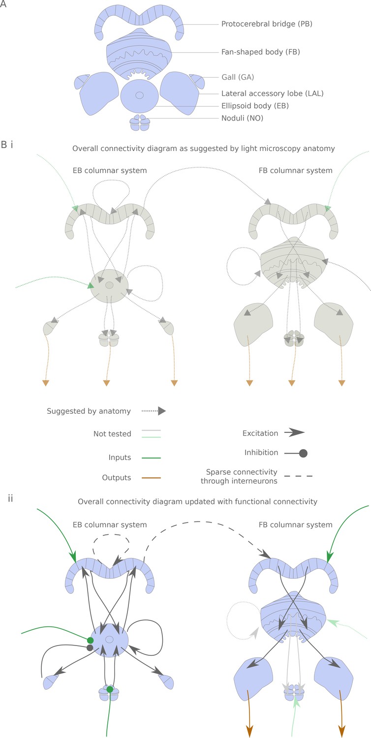
The central complex neuropiles and the hypothesized flow of information based on overlap of arbors in light-microscopy images.

(A) Schematic representation of the central complex and associated structures used throughout the manuscript. (B) (i) Hypothesized global information flow in the central complex based on neuron morphologies and the overlap of putative pre- and post-synaptic processes between different neuron types, based on Wolff et al. (2015) and Hanesch et al. (1989). (ii) Connectivity map based on the results of this study. Faded arrows represent hypotheses that were not tested in the present study.

https://doi.org/10.7554/eLife.37017.003

Figure 1—figure supplement 2

Download asset Open asset

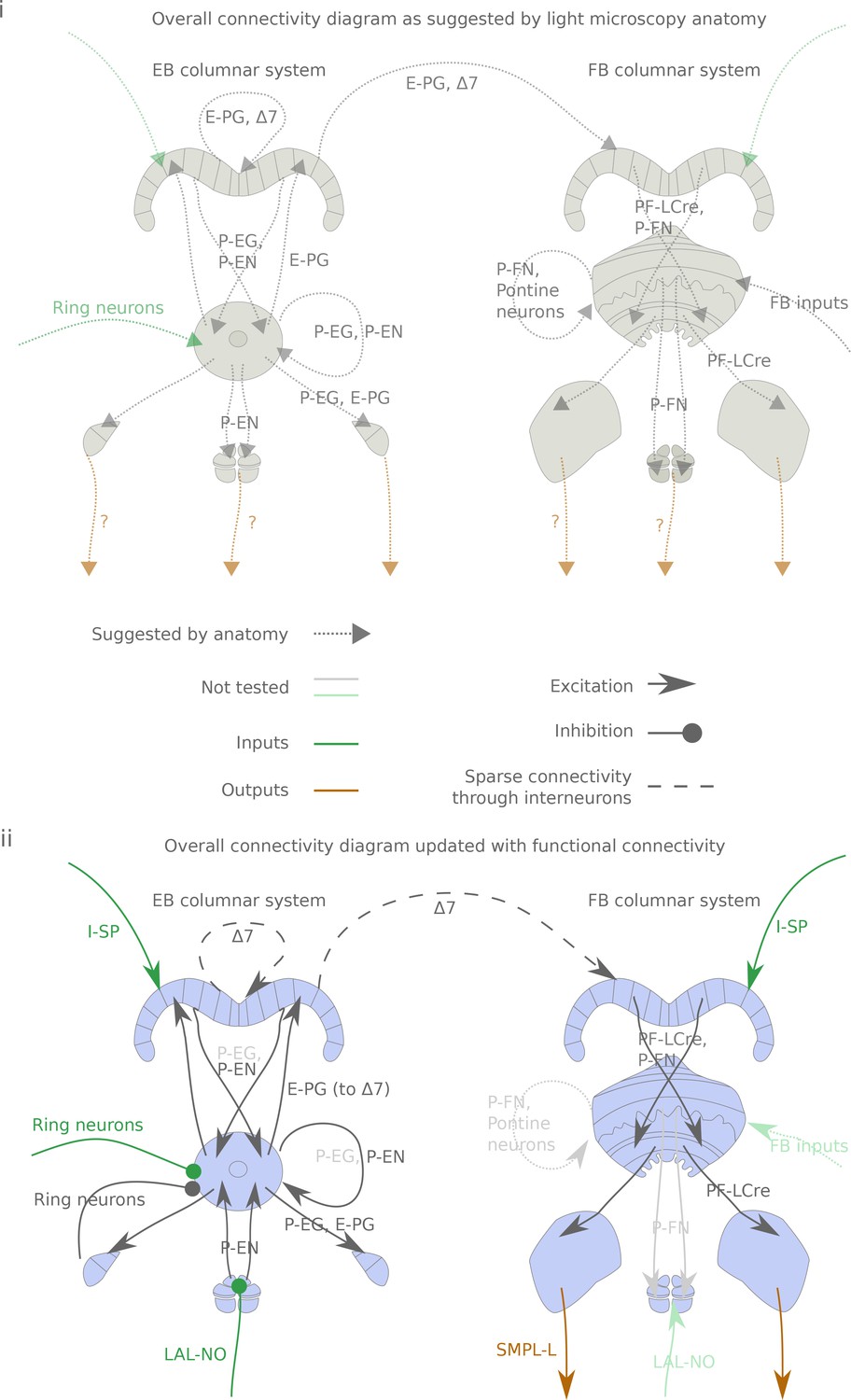
Same as figure Figure 1, but with neuron type names underlying the connections indicated.

Same as figure Figure 1, but with neuron type names underlying the connections indicated. (i) Hypothesized connections based on the anatomy described in Wolff et al. (2015) and Hanesch et al. (1989). (ii) Connectivity map based on the results of this study. Faded arrows and names represent hypotheses that were not tested in the present study.

https://doi.org/10.7554/eLife.37017.004

Figure 1—figure supplement 1

Download asset Open asset

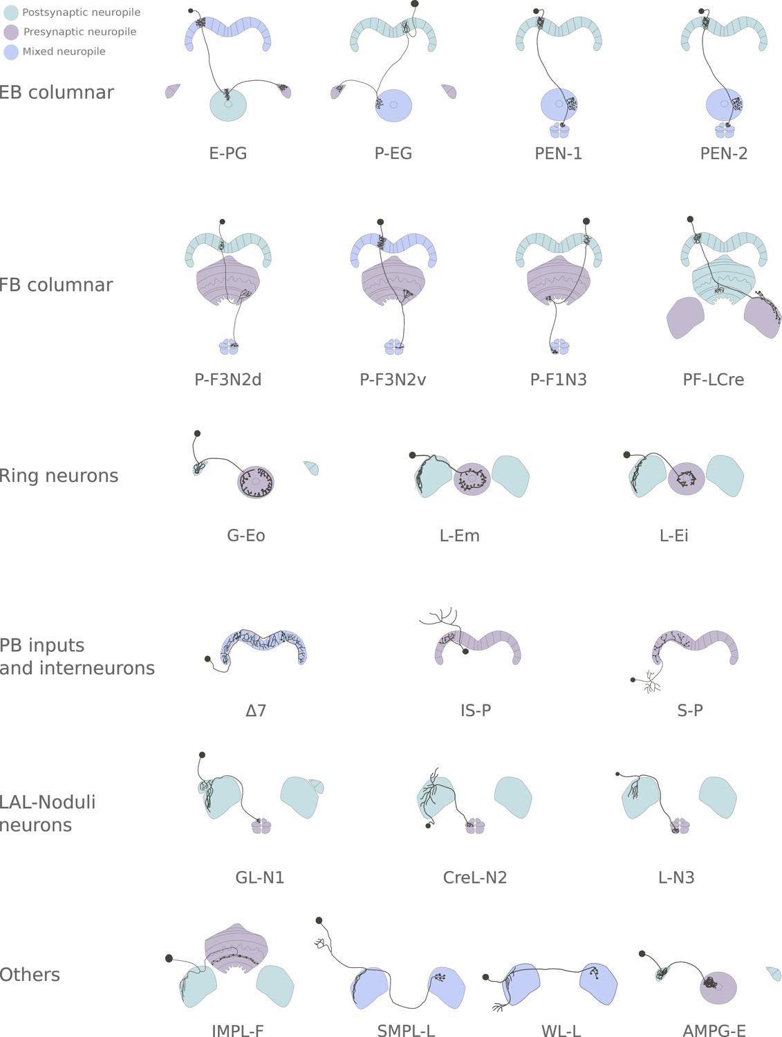
Diagrams of all the cell types used in the study.

Neuron types included in the study, grouped by super-type. P-EN1 and P-EN2 (Green et al., 2017) are drawn identically as they are almost indistinguishable based solely on anatomy. Note that each diagram represents a single neuron of the class. The driver lines selected contained most neurons of a given class. For columnar neuron classes, this meant that all or most columns were innervated.

https://doi.org/10.7554/eLife.37017.023

Figure 2

Download asset Open asset

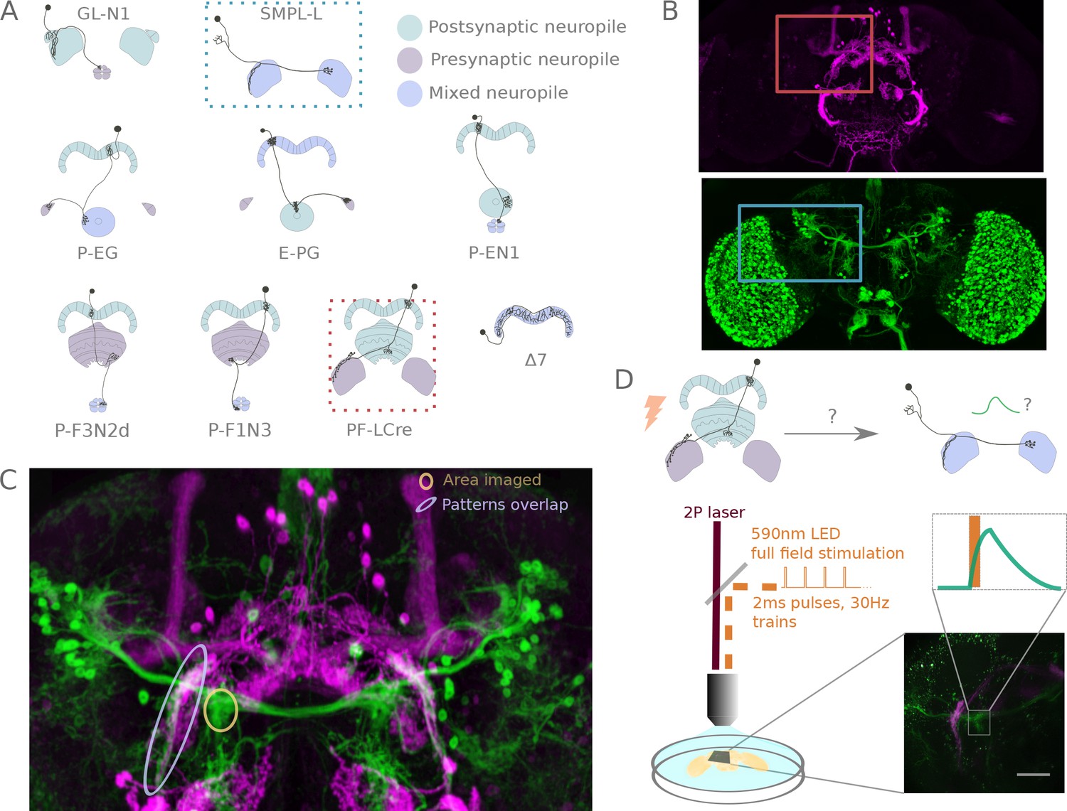
A functional connectivity screen.

(A) Schematics of a subset of the neurons considered for the screen. The example neurons shown in B, C and D are indicated by blue and orange dotted-line boxes. (B) For each potential neuronal pair, driver lines with clean expression in the central complex were selected — the boxes delineate the approximate position of the neurons of interest in the brain. (C) To determine if a given pair is a promising candidate, we examined the degree of overlap between putative pre- and post-synaptic regions in the expression patterns in anatomy images registered to a common brain template. If the candidate pre- and post-synaptic regions overlapped (as indicated by the blue ellipse), we expressed CsChrimson in the presynaptic candidate and GCaMP6m in the postsynaptic candidate, and then imaged the ex-vivo brain in a two-photon laser scanning microscope while optogenetically stimulating the candidate presynaptic population (D). We selected the region imaged based on proximity to the overlapping processes, but ensured that it contained only GCaMP expressing arbors (yellow ellipse in C, and box in D).

https://doi.org/10.7554/eLife.37017.007

Figure 3 with 6 supplements

Download asset Open asset

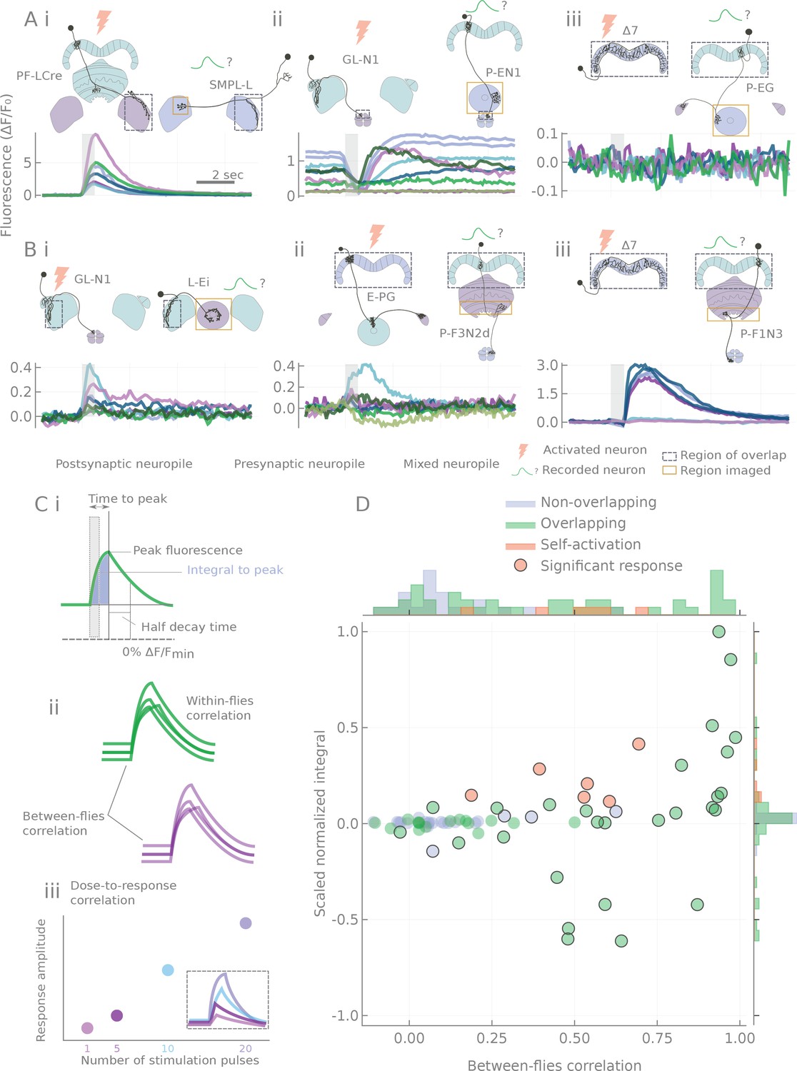
Characterization of calcium transients observed in response to o stimulation.

(**A and B**) Summary of different response types. Stimulation is indicated by the gray bar and consists of 20 light pulses (50 μW/mm², each of 2 ms duration) delivered at 30 Hz. (A) Example neuron pairs, easily interpretable responses. (B) Example neuron pairs, responses that are more difficult to interpret. In A and B, all responses, expressed as $Δ F / F_{0}$ , are baseline subtracted except for the inhibitory response in Aii. Scale bar 2 s. Grey dashed boxes show the region of overlap between the two patterns, and yellow boxes indicate the area that was generally imaged for the pairs shown. (C) Example of statistics computed on individual runs and cell pairs characterizing: (i) average response shape, (ii) reliability of the response, and (**iii**) response sensitivity. (D) Using the distribution of statistics from non-overlapping controls to assign classes to the responses: distributions of response amplitudes and reliability as measured by the scaled normalized integral (the median of the integral normalized to the baseline and scaled so that the dataset spans the [−1,1] range) and the between-flies correlation (see Materials and methods). Each point corresponds to a different cell pair (median statistics across flies). Control unconnected pairs are shown in blue, and self-activation (CsChrimson and GCaMP6m expressed in the same neuron type) in orange. Responses considered significantly different from the control sample (p<0.01, see Materials and methods) are circled.

https://doi.org/10.7554/eLife.37017.008

Figure 3—figure supplement 1

Download asset Open asset

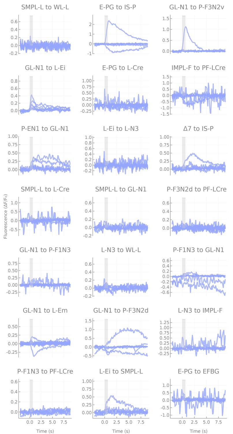
Responses of non-overlapping pairs.

Responses of non-overlapping pairs. Each line corresponds to a fly (six flies per pair), each panel to a cell pair tested. Note that when responses are present, they are either unreliable or small, and likely reflect effects of indirect connections.

https://doi.org/10.7554/eLife.37017.009

Figure 3—figure supplement 2

Download asset Open asset

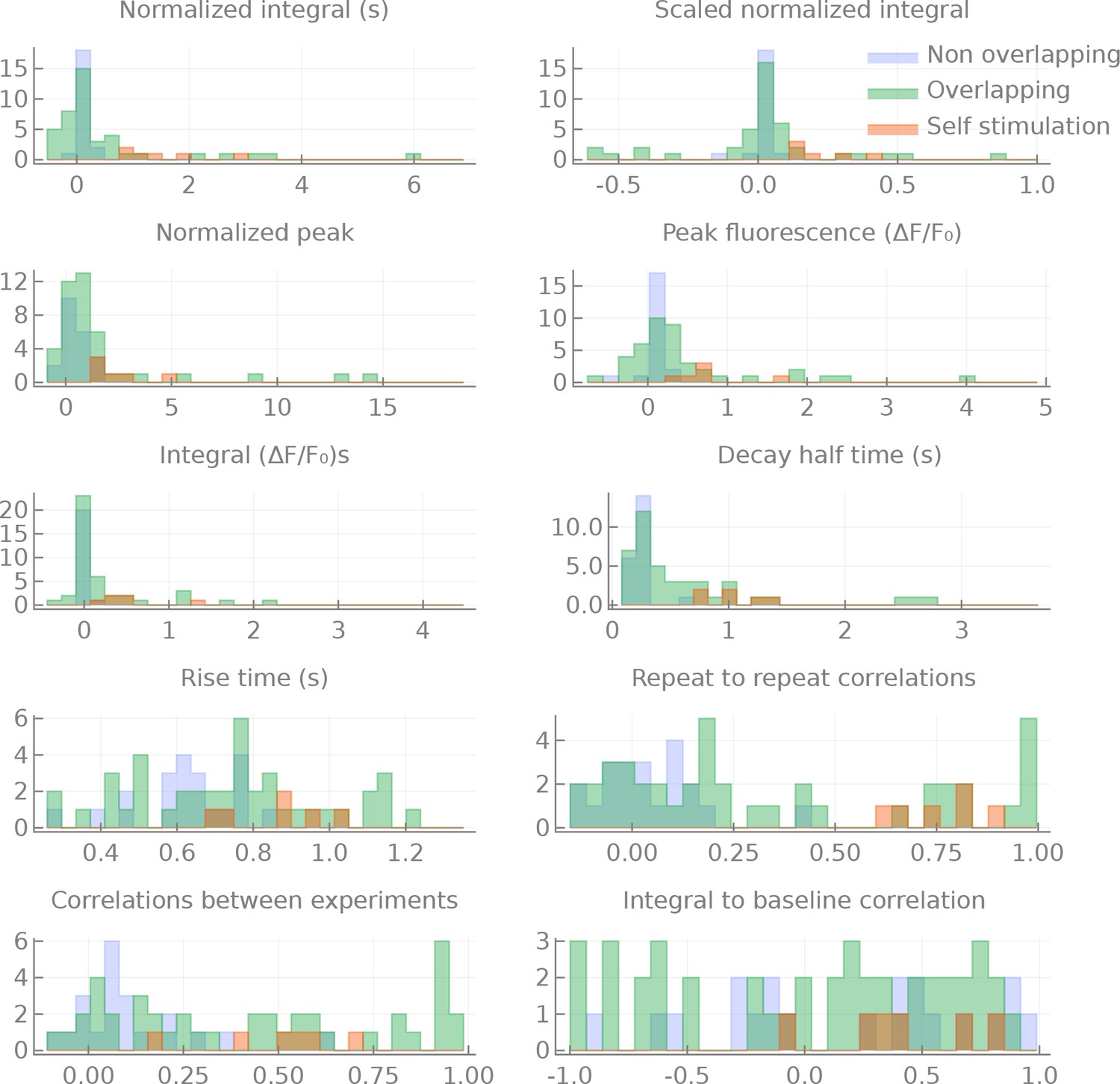
Distributions of the measured statistics for the different groups.

Distributions of statistics computed for non-overlapping, overlapping and self-activation pairs. All statistics are the median per pair of per run statistics. Integral: the integral of the response (from the onset of stimulation to the time of the peak of the response), in $Δ F / F_{0}$ s. Normalized integral: Integral divided by the baseline fluorescence. Scaled normalized integral: the normalized integral divided by the maximum (minimum for inhibitory responses) normalized integral measured. Peak fluorescence: the maximum (minimum for inhibitory responses) of the fluorescent transient $Δ F / F_{0}$ . Normalized peak: the peak fluorescence divided by the baseline fluorescence. Decay half time: the time in seconds between the peak of the response to the moment where the fluorescence reaches half the level of the peak (relative to the baseline). Rise time: the time of the peak fluorescence (in seconds). Repeat to repeat correlations: the average correlation between several repeats of the same experiment (in the same fly). Correlations between experiments: the average correlation between experimental runs of the same pair but from different flies. Integral to baseline correlation: the correlation between the integral and the value of the baseline fluorescence.

https://doi.org/10.7554/eLife.37017.010

Figure 3—figure supplement 3

Download asset Open asset

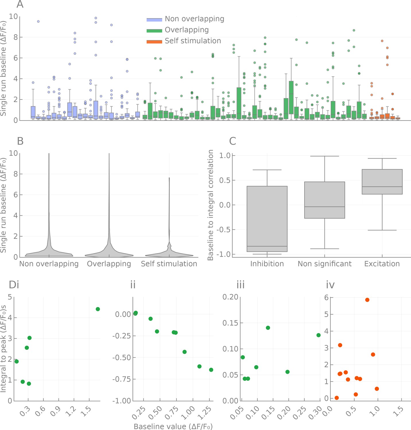
Effects of baseline fluorescence fluctuations on responses.

Spread of fluorescence baseline, effect on the responses. (A) Distribution of baseline fluorescence for each cell pair tested. Pairs are colored according to the ‘anatomical’ class they belong to (overlapping, non-overlapping and self-activation). (B) Same as A, but pooled by class and rendered as a violin plot. (C) Correlations between the signed response distance and the baseline fluorescence intensity of significantly responding pairs. Inhibitory responses are (as expected) correlated, but excitatory pairs also show a mild correlation. (D) Example of distance to baseline relationship in four pairs. (i) PF-LCre to SMPL-L, corresponding to Figure 3Ai. (ii) GL-N1 to P-EN1, corresponding to Figure 3Aii. (**iii**) GL-N1 to L-Ei, corresponding to Figure 3Aiii. (iv) PF-LCre to PF-LCre.

https://doi.org/10.7554/eLife.37017.011

Figure 3—video 1

Download asset

posterframe for video — PF-LCre to SMPL-L response, also shown in Ai.

Top left: average projection of the fluorescence movie with the outline of the ROI used to calculate the fluorescence. Top right: cell pair considered. The red box outlines the approximate location of the region imaged.

https://doi.org/10.7554/eLife.37017.012

Figure 3–video 2

Download asset

Figure 3–video 3

Download asset

Figure 4 with 5 supplements

Download asset Open asset

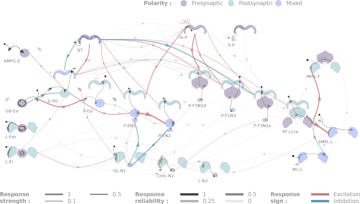
Diagrammatic representation of central complex connectivity.

Solid lines indicate anatomically overlapping cell pairs, whereas dotted lines correspond to the non-overlapping controls. The thickness of the lines maps to the functional connection strength. The reliability of the responses as measured by the between-flies correlations is mapped to the transparency of the connectors. Connection strengths are quantified in terms of the Mahalanobis distance to the null sample and the sign of the response integral, which is normalized to the maximum response. Three tested cell types (SMP-L2, L-Cre and EFBG) are not shown here for clarity, as tests with a few different partners did not produce significant results.

https://doi.org/10.7554/eLife.37017.015

Figure 4—figure supplement 1

Download asset Open asset

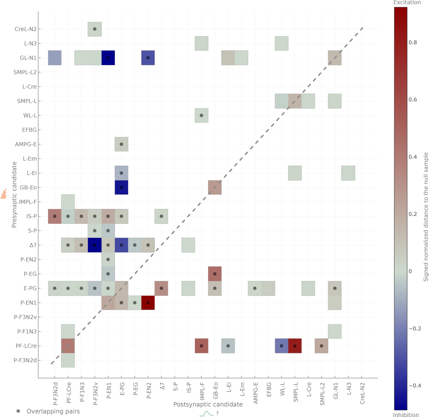
Matrix representation of the same data.

Matrix representation of the connectivity results. Dots denote anatomically overlapping pairs. The dashed diagonal correspond to self-activation (when the same cell expresses CsChrimson and GCaMP6m). Connection strengths are quantified in terms of the Mahalanobis distance to the null sample and the sign of the response integral, which is normalized to the maximum response.

https://doi.org/10.7554/eLife.37017.016

Figure 4—figure supplement 2

Download asset Open asset

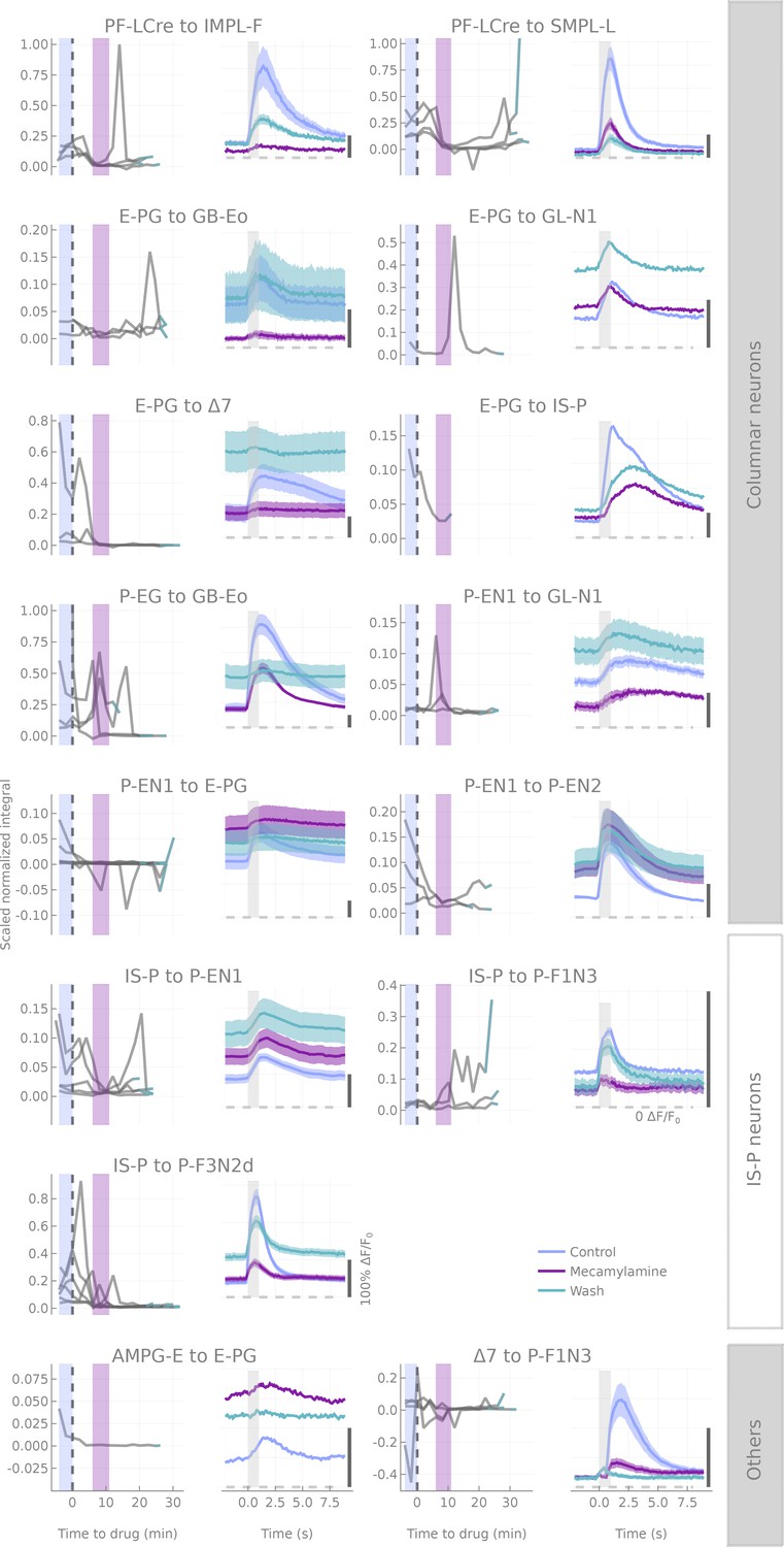
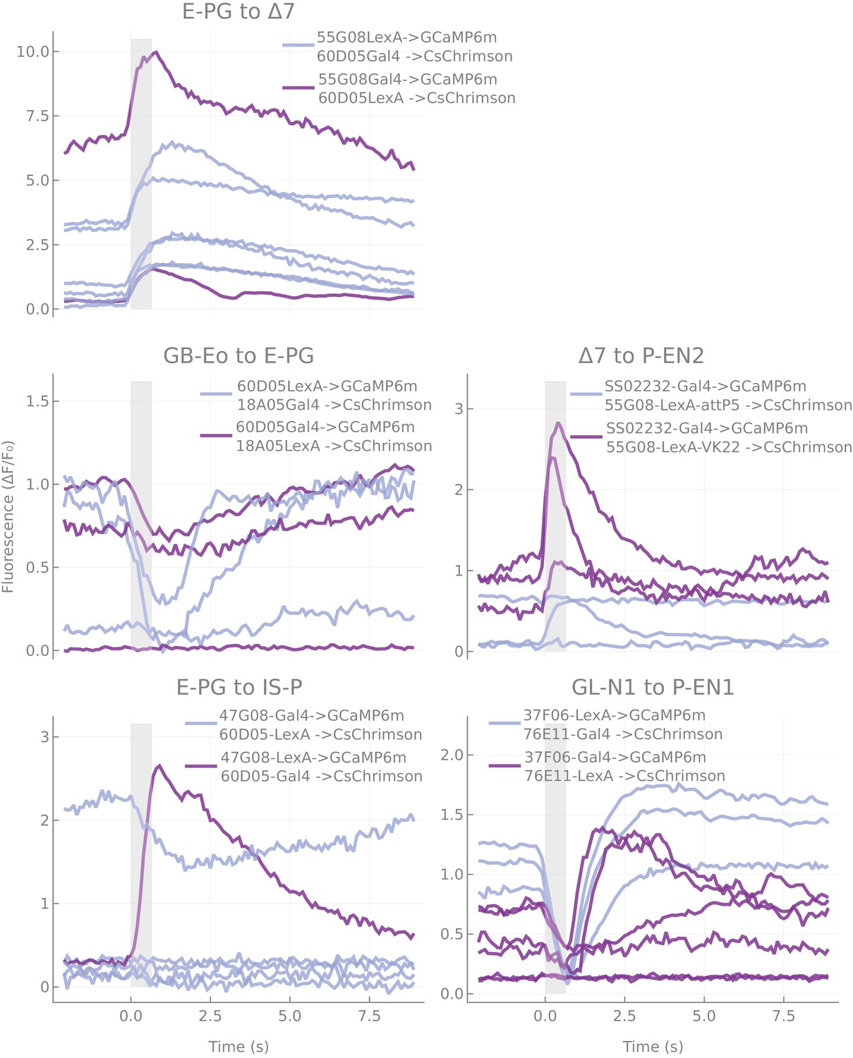
Results of mecamylamine applications.

For each cell pair, plots in the right column correspond to average traces (+-s.e.m.) at three time points during drug application: before (in blue, 4 min preceding drug application), during (in purple 6 to 11 min after starting drug application) and after (in turquoise, last two runs of the experiment). Plots in the left column show the response integral as a function of time to/from drug application. Each line corresponds to a fly. Timespans corresponding to the plots on the right are shaded accordingly. The dashed vertical line corresponds to the time at which the drug perfusion was turned on. Cell pairs are grouped based on the presynaptic cell type tested (Columnar neurons,IS-P neuron and Others).

https://doi.org/10.7554/eLife.37017.017

Figure 4—figure supplement 3

Download asset Open asset

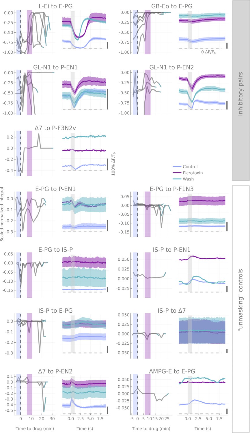
Results of picrotoxin applications.

Plots similar to Figure 4—figure supplement 2 for picrotoxin applications, except that experiments are now grouped based on the type of test that was run. ‘Inhibitory pairs’ show the straightforward assessment of inhibitory connections. Unmasking controls’ refers to attempts to uncover excitatory effects that might have been masked by global inhibition. Note that picrotoxin applications usually produce an increase in the baseline activity of the neuron, and hence an increase in the inhibitory driving force, which partially balances the transmission block.

https://doi.org/10.7554/eLife.37017.018

Figure 4—figure supplement 4

Download asset Open asset

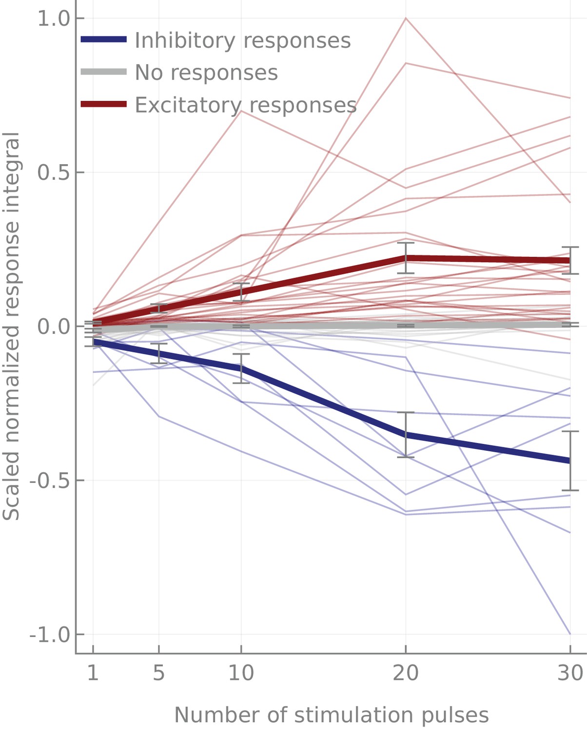
Dose response curves.

Dose responses. Thin lines correspond to median normalized scaled integrals of individual cell pairs. Cell pairs are grouped according to the class of their response (significantly excitatory/inhibitory or not significantly different from the controls). Note that both excitatory and inhibitory responses tend to saturate at 20 pulses.

https://doi.org/10.7554/eLife.37017.019

Figure 4—figure supplement 5

Download asset Open asset

Responses as a function of genotype used.

Responses of pairs for which several genotypes were tested.

https://doi.org/10.7554/eLife.37017.020

Figure 5 with 1 supplement

Download asset Open asset

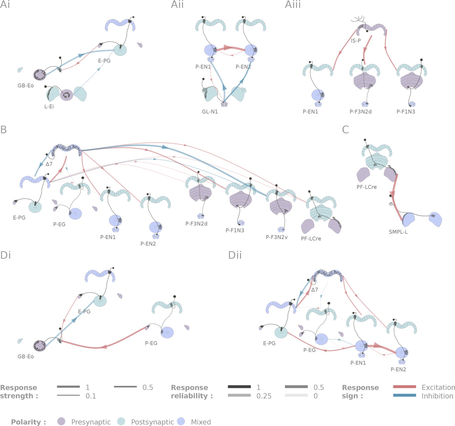
Selected connectivity motifs within the central complex.

(A) Input channels. (i) Ring neurons provide inhibitory input to the E-PGs in the EB. (ii) GL-N1 inhibits P-EN neurons. (**iii**) Distributed excitatory input from IS-P neurons in the PB. (B) $Δ$ 7 is probably the bottleneck in PB motifs, as it is the only strong post-synaptic target of E-PG neurons and relays information to other columnar neurons. (C) The only output pair found so far connects the PF-LCre neuron to a LAL interneuron. (D) Recurrence in the central complex. (i) at the input stage, and (ii) within the EB columnar system.

https://doi.org/10.7554/eLife.37017.021

Figure 5—figure supplement 1

Download asset Open asset

Various response types following $Δ$ 7 stimulation.

A: $Δ$ 7 to P-F3N2v, inhibitory. B: $Δ$ 7 to P-EN1, excitatory. C: $Δ$ 7 to E-PG, mixed responses. (i) to (iv) correspond to 5, 10, 20 and 30 pulses stimulation protocol. Each line is the average response for one fly (four runs per fly).

https://doi.org/10.7554/eLife.37017.022

Tables

Table 1

Drivers and neuron types used.

When the ‘Driver’ name is followed by an insertion site, it is a LexA line (see Materials and methods). Names starting by SS are stable splits. All other driver names correspond to both Gal4 (in attP2) and LexA (in attP40) drivers. ‘New Type Name’ refers to the nomenclature for short names adopted in this paper (following [Kakaria and de Bivort, 2017; Turner-Evans et al., 2017; Green et al., 2017]). Type description is the long name, following the guidelines of Wolff et al. (2015). Pre and post regions are labeled based on anatomical characteristics. The finer subdivisions were used to establish if two neurons were anatomically overlapping. The corresponding name in other insect species were determined using the insect brain database (https://insectbraindb.org/) and related papers (Heinze and Homberg, 2008; Heinze and Reppert, 2011b; Stone et al., 2017)

https://doi.org/10.7554/eLife.37017.005

Driver	New type name	Type description	Super type	Name in other insects
87G07	P-F3N2d	PBG2-9.s-FBl3.b-NO2D.b	FB columnar	CPU4 (b or c)
85H06	P-F1N3	PBG2-9.s-FBl1.b-NO3PM.b	FB columnar	CPU5
60D05	E-PG	PBG1-8.b-EBw.s-DV_GA.b	EB columnar	CL1a
SS02191	P-EG	PBG1-8.s-EBt.b-DV_GA.b	EB columnar	CL1b
67D09	P-F3N2v	PBG2-9.s-FBl3.b-NO2V.b	FB columnar	CPU4(a)
67D09-attP5	P-F3N2v	PBG2-9.s-FBl3.b-NO2V.b	FB columnar	CPU4(a)
67D09-VK22	P-F3N2v	PBG2-9.s-FBl3.b-NO2V.b	FB columnar	CPU4(a)
37F06	P-EN1	PBG2-9.s-EBt.b-NO1.b.Type1	EB columnar	CL2
37F06-VK22	P-EN1	PBG2-9.s-EBt.b-NO1.b.Type1	EB columnar	CL2
VT008135	P-EN1	PBG2-9.s-EBt.b-NO1.b.Type1	EB columnar	CL2
SS02232	P-EN2	PBG2-9.s-EBt.b-NO1.b.Type2	EB columnar	CL2
84H05	PF-LCre	PBG1-7.s-FBl2.s-LAL.b-cre.b	FB columnar	CPU1a
84H05-VK22	PF-LCre	PBG1-7.s-FBl2.s-LAL.b-cre.b	FB columnar	CPU1a
84H05-attP5	PF-LCre	PBG1-7.s-FBl2.s-LAL.b-cre.b	FB columnar	CPU1a
55G08	$Δ$ 7	PB18.s-Gx $Δ$ 7Gy.b-PB18.s-9i1i8c.b	PB interneuron	TB1
55G08-attP5	$Δ$ 7	PB18.s-Gx $Δ$ 7Gy.b-PB18.s-9i1i8c.b	PB interneuron	TB1
55G08-VK22	$Δ$ 7	PB18.s-Gx $Δ$ 7Gy.b-PB18.s-9i1i8c.b	PB interneuron	TB1
47G08	IS-P	PBG2-9.b-IB.s.SPS.s	PB input
49H05	IMPL-F	LAL.s-IMP-FBl3.b	FB input
75H04	L-Ei	EBIRP I-O-LAL.s	Ring neuron	TL4
32A11	L-Em	EBMRP I-O-LAL.s	Ring neuron	TL4
18A05	GB-Eo	EBORP O-I-GA-Bulb	Ring neuron
18A05-VK22	GB-Eo	EBORP O-I-GA-Bulb	Ring neuron
17H12	AMPG-E	EB.w-AMP.d-D_GAsurround	EB input
12C11	EFBG	EBMRA-FB-LT-LT-GA-GA	Other
72H06	SMPL-L	SMP.s-LAL.s-LAL.b.contra	LAL-IN
72H06-attP5	SMPL-L	SMP.s-LAL.s-LAL.b.contra	LAL-IN
72H06-VK22	SMPL-L	SMP.s-LAL.s-LAL.b.contra	LAL-IN
SS02615	SMPL-L2	SMP.s-LAL.s-LAL.b.contra2	LAL-IN
26B07	WL-L	Wedge-LAL.s-LAL.b.contra	LAL-IN
31A11	L-Cre	LAL-Cre	LAL-IN
SS00153	S-P	SPS.s-PB.b	PB input
76E11	GL-N1	LAL.s-GAi.s-NO1i.b	LAL-NO
76E11-VK22	GL-N1	LAL.s-GAi.s-NO1i.b	LAL-NO
SS04448	GL-N1	LAL.s-GAi.s-NO1i.b	LAL-NO
SS04420	CreL-N2	Cre.s-LAL.s-NO2.b	LAL-NO	TN1 ?
12G04	L-N3	LAL.s-NO3Ai.b	LAL-NO	TN1 ?

Table 2

Number of cells per hemisphere and PB column (when relevant) in the drivers used in this study, as estimated by counting cell bodies in confocal stacks.

When counting was difficult (e.g. because of densely packed somata) we indicated this by a $\sim$ sign.

https://doi.org/10.7554/eLife.37017.006

Driver	New type name	Cells per hemisphere	Cells per column
87G07	P-F3N2d	16	2
85H06	P-F1N3	32	4
60D05	E-PG	24	3
SS02191	P-EG	16	2
67D09	P-F3N2v	24	3
37F06	P-EN1	24	3
VT008135	P-EN1	24	3
SS02232	P-EN2	16	2
84H05	PF-LCre	7	1
55G08	$Δ$ 7	16
47G08	IS-P	12
49H05	IMPL-F	4
75H04	L-Ei	$\sim$ 30
32A11	L-Em	$\sim$ 24
18A05	GB-Eo	2
17H12	AMPG-E	$\sim$ 12
12C11	EFBG	9
72H06	SMPL-L	$\sim$ 12
SS02615	SMPL-L2	$\sim$ 12
26B07	WL-L	2
31A11	L-Cre	2
SS00153	S-P	2
76E11	GL-N1	2
SS04448	GL-N1	2
SS04420	CreL-N2	2
12G04	L-N3	2

Additional files

Supplementary file 1 Summary table of experiments. The table contains condensed information about the individual experiments: Cell Pair: the cell pair tested, genotype: the LexA, Gal4 and expression system driving CsChrimson (enough to reconstruct the full genotype, see Materials and methods, region imaged: the neuropile imaged for a given experiment. in or out suffixes denote that the processes entering (exiting) the neuropile were imaged, data folder: the raw data folder corresponding to that experiment in the OpenScienceFramework project (https://osf.io/vsa3z/), Stack: the number corresponding to the anatomical stack for that experiment in the previously identified data folder.: https://doi.org/10.7554/eLife.37017.024
Download elife-37017-supp1-v2.csv
Transparent reporting form: https://doi.org/10.7554/eLife.37017.025
Download elife-37017-transrepform-v2.docx