Sparse recurrent excitatory connectivity in the microcircuit of the adult mouse and human cortex
- Allen Institute for Brain Science, United States
- Regional Epilepsy Center at Harborview Medical Center, United States
- University of Washington School of Medicine, United States
- Swedish Neuroscience Institute, United States
Figures
Figure 1 with 1 supplement

Electrophysiological recordings of evoked excitatory synaptic responses between individual cortical pyramidal neurons in mouse primary visual cortex.
(A) Cartoon illustrating color, Cre-line, and cortical layer mapping in slice recording region (V1). Example maximum intensity projection images of biocytin-filled pyramidal neurons for L2/3 and each Cre line. (B) Example epifluorescent images of neurons showing Cre-dependent reporter expression and/or dye-filled recording pipettes. Connection map is overlaid on the epifluorescent image (colored: example connection shown in C). (C) Spike time aligned EPSPs induced by the first AP of all ≤ 50 Hz stimulus trains for a single example connection (individual pulse-response trials: grey; average: colored). (D) First pulse average, like in C., for all connections within the synaptic type; grey: individual connections; thin-colored: connection highlighted in C; thick-colored: grand average of all connections. (E) Overlay of grand average for each connection type. (F) EPSP amplitude (in log units), CV of amplitude, latency, and rise time of first-pulse responses for each Cre-type (small circles) with the grand median (large). See Figure 1—figure supplement 1 for data processing and analysis diagrams.
-
Figure 1—source data 1
Electrophysiological recordings of evoked excitatory synaptic responses between individual cortical pyramidal neurons in mouse primary visual cortex.
- https://doi.org/10.7554/eLife.37349.006
Figure 1—figure supplement 1
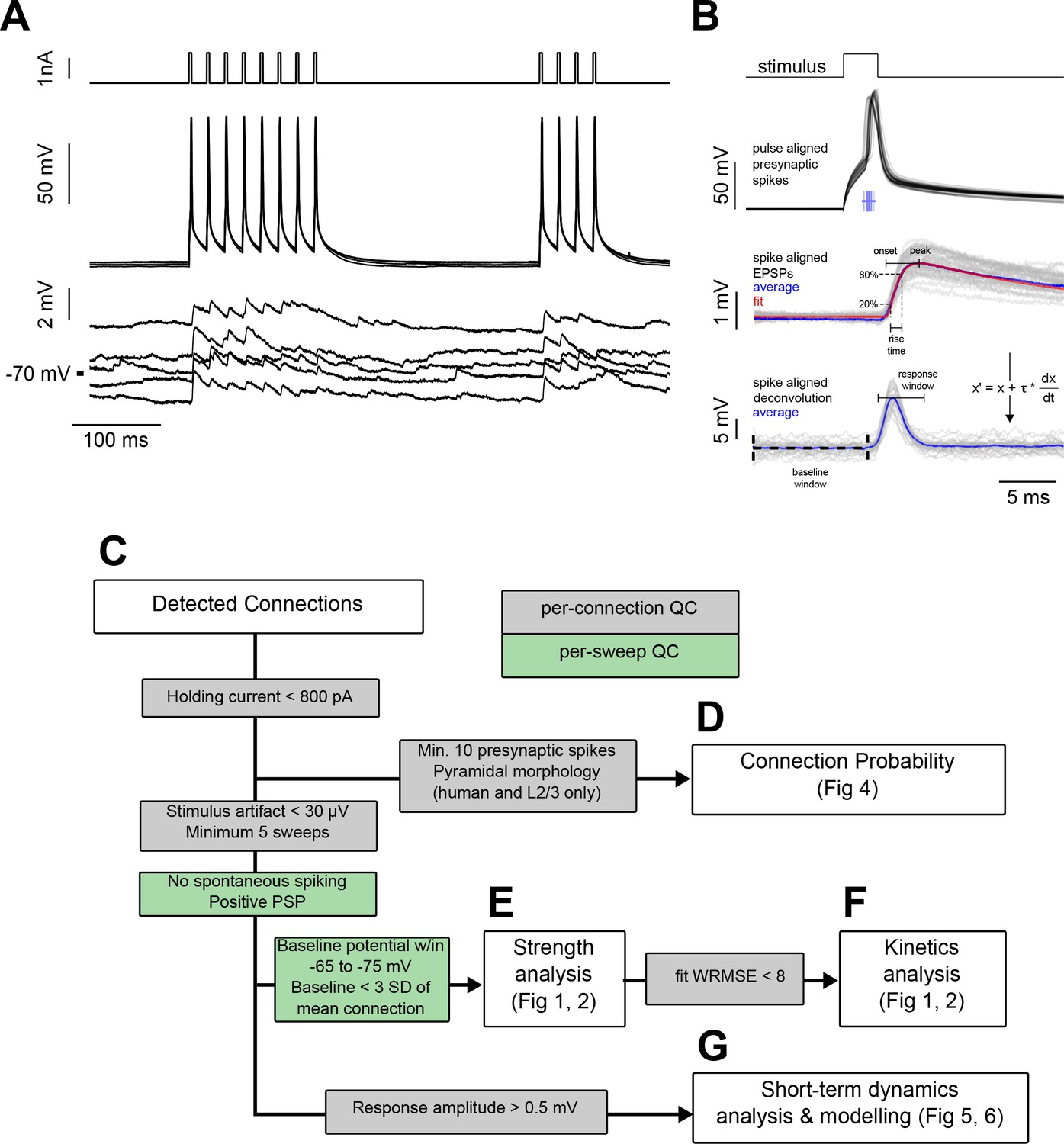
Experiment methodology and analysis workflow.
(A) Example connected pair showing the stimulation pulses (top) and action potentials (middle) in the presynaptic cell; monosynaptically evoked EPSPs (bottom) in the postsynaptic cell. Traces represent every fifth sweep from the 50 Hz protocol used to measure recovery from STP at a delay of 250 ms. (B) Following repeated stimulation, the response to the first spike in each train of current pulsess was used for EPSP feature analysis. Spikes are shown aligned to the pulse time to illustrate jitter in spike timing. Spike time was defined as the region of maximum dV/dt in the spike trace, as shown in the raster plot corresponding to spike timing of individual spikes. Below, EPSPs are aligned to the spike time prior to fitting the average EPSP (see Equation 1; individual sweeps in grey, average response in blue, fit shown in red). The rise time was calculated as the interval between 20% and 80% of the peak amplitude of the fit. Spike-aligned EPSPs were deconvolved (see Equation 2, shown in figure), and the peak amplitudes of the deconvolved traces were used to measure changes in response amplitude of the course of a spike train. Responses were corrected to the baseline by subtracting the mode of the region between 10 ms and 50 µs prior to stimulus onset (baseline window). Responses were measured as the peak response during a 4 ms window beginning 1 ms after the spike time (response window shown is aligned to mean spike time). (C–G) Subsets of total connectivity data were used in subsequent analysis. Flowchart shows sweep (green) and connection (grey) level inclusion criteria for data included in each figure. See Table 1 for total number of cells in each criterion.
Figure 2

Electrophysiological recordings of evoked excitatory synaptic responses between individual human cortical pyramidal neurons.
(A) Cartoon illustrating color and cortical layer mapping in slice recording region (temporal or frontal cortex). Example maximum intensity projection images of biocytin-filled pyramidal neurons for layers 2–5. (B) Example epifluorescent images of neurons showing dye-filled neurons and recording pipettes. Connection map is overlaid on the epifluorescent image (colored: example connection shown in C). (C) Spike time aligned EPSPs induced by the first AP of all ≤ 50 Hz stimulus trains for a single example connection (individual pulse-response trials: grey; average: colored). (D) First pulse average, like in C., for all connections within the synaptic type; grey: individual connections; thin-colored: connection highlighted in C; thick-colored: grand average of all connections. (E) Overlay of grand average for each connection type. (F) EPSP amplitude, CV of amplitude, latency, and rise time of first-pulse responses for each layer (small circles) with the grand mean (large circles). See Figure 1—figure supplement 1 for data processing and analysis diagrams.
-
Figure 2—source data 1
Electrophysiological recordings of evoked excitatory synaptic responses between individual human cortical pyramidal neurons.
- https://doi.org/10.7554/eLife.37349.009
Figure 3

Characterization of synapse detection limits.
(A) Scatter plot showing measured EPSP amplitude versus minimum detectable amplitude for each tested pair. Detected synapses (manually annotated) are shown as blue diamonds; pairs with no detected EPSPs are grey dots. The region under the red dashed line denotes the region in which synaptic connections are likely to be misclassified as unconnected. Three example putative connections are highlighted in A and described further in panels B-D. One connection (top row) was selected for its large amplitude PSP and low background noise. Another connection (middle row) is harder to detect (PSP onset marked by yellow arrowhead) due to low amplitude and high background noise. The bottom row shows a recorded pair that was classified as unconnected. (B) A selection of postsynaptic current clamp recordings in response to presynaptic spikes. Each row contains recordings from a single tested pair. The vertical line indicates the time of presynaptic spikes, measured as the point of maximum dV/dt in the presynaptic recording. Yellow triangles indicate the onset of the EPSP. (C) Histograms showing distributions of peak response values measured from deconvolved traces (see Materials and methods). Red area indicates measurements made on background noise; blue area indicates measurements made immediately following a presynaptic spike. (D) Characterization of detection limits for each example. Plots show the probability that simulated EPSPs would be detected by a classifier, as a function of the rise time and mean amplitude of the EPSPs. Each example has a different characteristic detection limit that depends on the recording background noise and the length of the experiment. (E) An estimate of the total number of false negatives across the entire dataset. The measured distribution of EPSP amplitudes is shown in light grey (smoothed with a Gaussian filter with σ = 1 bin). The estimated correction show in dark grey is derived by dividing the measured distribution by the overall probability of detecting a synapse (red dashed line) at each amplitude. See Supplementary file 1 for features included in classifier.
-
Figure 3—source data 1
Characterization of synapse detection limits.
- https://doi.org/10.7554/eLife.37349.012
Figure 4 with 3 supplements
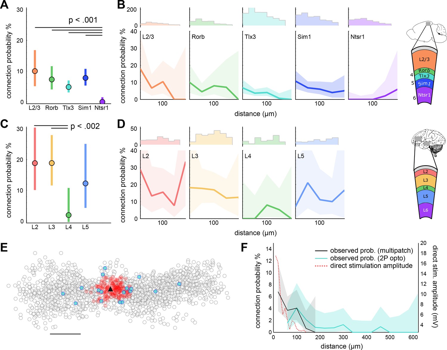
Distance dependent connectivity profiles of mouse and human E-E connections.
(A) Recurrent connection probability and distribution of connections for mouse -linesand layer 2/3. Mean connection probability (filled circles) and 95% confidence intervals (bars) for connections probed within 100 µm (n connections in Table 1). (B) Connection probability over distance for mouse Cre-lines and layer 2/3. Top: Histogram of putative connections probed. Bottom: Mean connection probability (thick line) with 95% confidence intervals (shading) binned in 40 µm increments. (C) Like-to-like connection probability and distribution of connections between human pyramidal neurons. Mean connection probability (filled circles) and 95% confidence intervals (bars) for connections probed within 100 µm. (D) Connection probability over distance for human pyramidal neurons, formatted as in panel B. (E) Tlx3-Tlx3 connection probability measured by two-photon mapping. X-Y distance distribution of connections probed onto a postsynaptic cell (black triangle), detected presynaptic neurons (filled circles), no connection detected (empty circles), and direct event artifact due to undesired activation of opsin in the dendritic arbor of the recorded cell (red circles). (F) Connection probability and stimulation artifact over distance measured by two-photon mapping. Mean connection probability vs. distance (blue line; starting at 50 µm) with 95% confidence intervals (shading) and direct event artifact amplitude vs. distance (dotted red line) for Tlx3-Tlx3 connections probed with two-photon stimulation. See Figure 4—figure supplement 3 for distribution of connectivity as a function of cortical slice position and cell depth. See Figure 4—figure supplements 1,2 for details on two-photon connectivity experiments.
-
Figure 4—source data 1
Distance dependent connectivity profiles of mouse and human E-E connections.
- https://doi.org/10.7554/eLife.37349.017
Figure 4—figure supplement 1

Intralaminar connectivity rates were unaffected by recording depth and medial-lateral position in V1.
(A) Connectivity rate was assessed as a function of slice number, spanning a total sampled region across experiments of 3.5 mm of cortex (350 µm per slice). (B) The observed synaptic connectivity (open circles) and 95% CI (grey region) are shown relative to overall average connectivity (dotted line). (C) Connectivity was not influenced by depth from the slice surface between −40 and −200 µm. Sampling frequency and connectivity as a function of depth from slice surface are shown in D.
-
Figure 4—figure supplement 1—source data 1
Intralaminar connectivity rates were unaffected by recording depth and medial-lateral position in V1.
- https://doi.org/10.7554/eLife.37349.018
Figure 4—figure supplement 2

Characterization of two-photon photostimulation.
(A) Cartoon illustrating loose-seal recording configuration utilized to test photostimulation parameters. Example recording of repeated photostimulation or a ReaChR-positive cell. (B) Cumulative probability plot of minimum power necessary to reliably evoke action potentials for 13 cells. Blue dashed lines indicate light power utilized in mapping experiments and the fraction of cells reliably activated. (C) Average latency of light-evoked action potentials plotted against photostimulation intensity for individual neurons (grey dashed lines). Filled black circle and error bars represent the mean and standard deviation of latency measured across all cells at a power used for mapping. (D) Average jitter of light-evoked action potentials plotted against photostimulation intensity. Data from individual cells and population average plotted as in panel C. (E) Left: Example experiment illustrating the radial grid pattern used to measure the lateral resolution of photostimulation and example traces recorded during the photostimulation at indicated locations. Right: Probability of generating light-evoked action potentials plotted against lateral distance from the center of the cell. (F) Left: example of responses resulting from photostimulation at indicated axial offsets. Right: Probability of generating light-evoked action potentials plotted against axial distance from the center of the cell.
-
Figure 4—figure supplement 2—source data 1
Characterization of two-photon photostimulation.
- https://doi.org/10.7554/eLife.37349.019
Figure 4—figure supplement 3
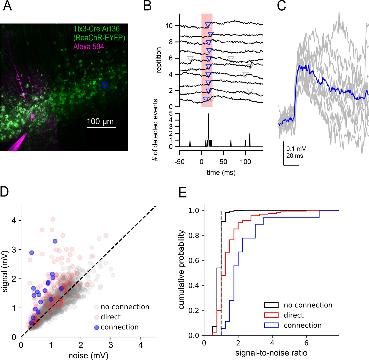
Two-photon optogenetic mapping details.
(A) Maximum intensity projection of Tlx3-Cre:Ai136 slice and a recorded neuron. Blue circle denotes location of stimulated presynaptic neuron. (B) Top: Electrophysiological recording of postsynaptic response to 10 photostimulations of the presynaptic neuron in panel A. Timing of photostimulation indicated by pink shading. Synaptic events detected by exponential deconvolution are indicated by inverted triangles. Events used to produce average synaptic response are show in blue. Bottom: Peri-stimulus event histogram. (C) Individual events aligned by the timing of event detection (grey) and average EPSP (blue). (D) Signal versus noise plot for all optogenetically-probed presynaptic neurons. (E) Cumulative probability plot of signal-to-noise ratios for stimulus trials scored as no connection, connection, or containing a direct stimulation artifact. Dashed grey line indicates signal-to-noise ratio = 1.
-
Figure 4—figure supplement 3—source data 1
Two-photon optogenetic mapping details.
- https://doi.org/10.7554/eLife.37349.020
Figure 5 with 1 supplement
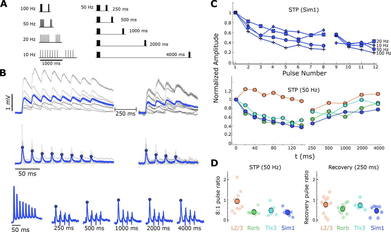
Short-term dynamics of mouse recurrent connections by Cre-line and layer (n in Table 1 ‘STP’).
(A) Schematic of STP and STP recovery stimuli. (B) Sim1-Cre EPSPs in response to a 50 Hz stimulus train (top; eight induction pulses and four recovery pulses delayed 250 ms; individual connection: gray traces; blue: Sim1-Cre average EPSP at 50 Hz). Exponential deconvolution followed by lowpass filter of EPSPs above (middle, filled circles: pulse amplitudes in C). Exponential deconvolution of 50 Hz stimulus with all five recovery time points in A (bottom, filled circles: pulse amplitudes in C). (C) The mean normalized amplitude of deconvolved response versus pulse number at multiple stimulation frequencies for Sim1-Cre (top). Normalized amplitude of the deconvolved response at 50 Hz with first recovery pulse at each interval for each Cre-line and L2/3 connections (bottom). (D) The depth of depression during 50 Hz induction (left) as measured by the amplitude ratio of the 8th to 1st pulse for each Cre-line and layer (small circles) and grand mean (large circles). Amount of recovery at 250 ms latency (right) for each Cre-line and layer (small circles) and grand mean (large circles). See Figure 5—figure supplement 1 for results of STP at different EGTA concentrations and Figure 1—figure supplement 1 for data analysis diagram.
-
Figure 5—source data 1
Influence of internal EGTA on short-term dynamics.
- https://doi.org/10.7554/eLife.37349.023
Figure 5—figure supplement 1

Influence of internal EGTA on short-term dynamics.
(A) Normalized response amplitude during a 50 Hz train in Tlx3 (cyan) and Sim1 (blue) connections with 0.3 mM EGTA present in the internal solution (filled) and in the absence of EGTA (open). Data are grand average of all connections within each type. (B) Ratio of the last (8th) pulse in the train to the first for each connection within each type (small circles) and the grand mean (large circle); colors and fill follow as in A. (C) Paired-pulse ratio for each connection within each type (small circles) and the grand mean (large circles); colors and fill follow as in A.
-
Figure 5—figure supplement 1—source data 1
Influence of internal EGTA on short-term dynamics.
- https://doi.org/10.7554/eLife.37349.024
Figure 6
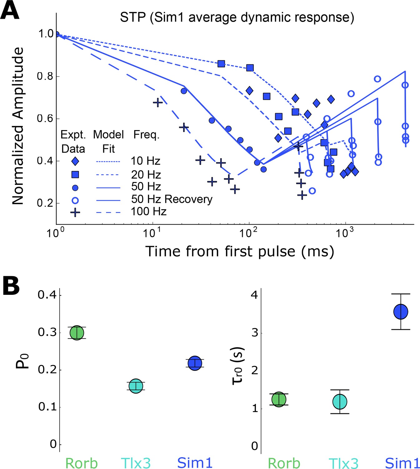
Modeling of short-term depression in recurrent Rorb, Sim1, and Tlx3 connections (n in Table 1 ‘STP’).
(A) Sim1 average dynamic response; Same data as in Figure 5C, top plotted on a log-X time scale with modeling fits overlaid. (B) Results of model for parameters P0 and 𝜏r0. Values are means with standard error of the covariance matrix. Paired Z-scores (Equation 6) in Table 5.
Tables
Table 1
The number of connections probed and the number of connections used in subsequent analyses per the analysis flow diagram in Figure 1—figure supplement 1C–G.
For each column, the Figure 1—figure supplement 1 letter indicates the end level in the analysis flow diagram while the main figure reference indicates n connections included in that figure. For example, the ‘Strength’ column indicates the number of connections for each type used to measure the strength (or amplitude) of the connection as shown in Figure 1F. The inclusion criteria for these connections can be followed in the diagram in Figure 1—figure supplement 1E. Similarly, these data are provided for kinetics (rise time and latency) and short-term plasticity (STP).
| Layer/Cell Type | Total probed (Figure 1—figure supplement 1C) | Total connected (Figure 1—figure supplement 1C) | Total connection probability (%) | Strength (Figure 1—figure supplement 1E, Figure 1F) | Kinetics (Figure 1—figure supplement 1F, Figure 1F) | Connection probability (%) w/in 100 µm (Connected/probed, Figure 1—figure supplement 1D, Figure 4A,C) | STP (Figure 1—figure supplement 1G, Figures 5 and 6) |
|---|---|---|---|---|---|---|---|
| Mouse L2/3 | 180 | 15 | 8.3 | 12 | 9 | 13/130 (10.0) | 9 |
| Rorb | 315 | 20 | 6.3 | 13 | 13 | 18/247 (7.3) | 9 |
| Tlx3 | 1108 | 39 | 3.5 | 17 | 14 | 36/746 (4.8) | 5 |
| Sim1 | 783 | 55 | 7.0 | 18 | 18 | 41/527 (7.8) | 7 |
| Ntsr1 | 450 | 2 | 0.4 | 2 | 2 | 0/313 (0.0) | N/A |
| Human L2 | 132 | 22 | 16.7 | 18 | 18 | 13/69 (18.8) | N/A |
| Human L3 | 249 | 37 | 14.9 | 33 | 29 | 20/106 (18.9) | N/A |
| Human L4 | 123 | 4 | 3.3 | 2 | 2 | 1/51 (2.0) | N/A |
| Human L5 | 112 | 13 | 11.6 | 6 | 6 | 6/49 (12.2) | N/A |
Table 2
Properties of mouse EPSPs.
Median, mean, and standard deviation of EPSP properties plotted in Figure 1F for each layer and Cre-type. Number of connections used in the amplitude and CV analysis are found in Table 1 ‘Strength’, or for latency and rise time in Table 1 ‘Kinetics’.
| Amp median (mV) | Amp mean (mV) | Amp SD (mV) | Latency median (ms) | Latency mean (ms) | Latency SD (ms) | Rise Time median (ms) | Rise Time mean (ms) | Rise Time SD (ms) | CV median | CV mean | CV SD | |
|---|---|---|---|---|---|---|---|---|---|---|---|---|
| L2/3 | 0.26 | 0.34 | ±0.32 | 1.48 | 1.87 | ±1.0 | 1.24 | 1.45 | ±0.57 | 0.55 | 0.56 | ±0.15 |
| Rorb | 0.31 | 0.54 | ±0.49 | 1.31 | 1.50 | ±0.6 | 1.32 | 1.63 | ±0.94 | 0.59 | 0.55 | ±0.24 |
| Sim1 | 0.33 | 0.52 | ±0.51 | 1.86 | 2.05 | ±0.82 | 1.91 | 1.86 | ±1.1 | 0.36 | 0.43 | ±0.2 |
| Tlx3 | 0.14 | 0.24 | ±0.24 | 1.81 | 2.07 | ±0.74 | 1.44 | 1.35 | ±1.1 | 0.51 | 0.51 | ±0.18 |
Table 3
Properties of human EPSPs.
Median, mean, and standard deviation of EPSP properties plotted in Figure 1F for each layer and Cre-line. Number of connections used in the amplitude and CV analysis are found in Table 1 ‘Strength’, for latency and rise time in Table 1 ‘Kinetics’.
| Amp median (mV) | Amp mean (mV) | Amp SD (mV) | Latency median (ms) | Latency mean (ms) | Latency SD (ms) | Rise time median (ms) | Rise time mean (ms) | Rise time SD (ms) | CV median | CV mean | CV sd | |
|---|---|---|---|---|---|---|---|---|---|---|---|---|
| L2 | 0.22 | 0.30 | ±0.22 | 1.84 | 1.79 | ±0.78 | 1.47 | 1.53 | ±0.59 | 0.80 | 0.64 | ±0.29 |
| L3 | 0.34 | 0.54 | ±0.68 | 1.57 | 1.58 | ±0.97 | 1.60 | 2.07 | ±1.36 | 0.39 | 0.44 | ±0.23 |
| L4 | 0.97 | 0.97 | ±1.05 | 2.70 | 2.70 | ±1.80 | 2.02 | 2.02 | ±0.47 | 0.37 | 0.37 | ±0.20 |
| L5 | 0.62 | 0.80 | ±0.69 | 1.64 | 1.75 | ±0.59 | 1.16 | 1.23 | ±0.46 | 0.29 | 0.34 | ±0.10 |
Table 4
Mean and standard deviation of 8:1 ratio at 50 Hz and 9:1 ratio at 50 Hz and 250 ms delay for individual synapses.
Unless noted, EGTA was 0.3 mM and n’s are listed in Table 1, STP.
| 8:1 pulse ratio (50 Hz) mean ± SD | Recovery (9:1) ratio (250 ms) mean ± SD | Paired-pulse ratio (50 Hz) mean ± SD | |
|---|---|---|---|
| L2/3 | 0.92 ± 0.57 | 0.76 ± 0.48 | 1.14 ± 0.63 |
| Rorb | 0.39 ± 0.14 | 0.55 ± 0.26 | 0.66 ± 0.13 |
| Sim1 | 0.37 ± 0.18 | 0.46 ± 0.26 | 0.73 ± 0.17 |
| Tlx3 | 0.48 ± 0.32 | 0.72 ± 0.24 | 0.8 ± 0.15 |
| Sim1 (0 EGTA), n = 6 | 0.27 ± 0.17 | N/A | 0.68 ± 0.22 |
| Tlx3 (0 EGTA), n = 2 | 0.51 ± 0.12 | N/A | 1.15 ± 0.03 |
Table 5
Model parameter values and statistics for Rorb, Sim1, and Tlx3 recurrent connections.
Parameter values are from the model performed on the grand mean for each connection type with the standard error of the covariance matrix. The Z-score was computed following Equation 6; the Z-score between each possible pair should be read as a matrix with the corresponding Cre-line in the row. Number of connections used in this analysis in Table 1 ‘STP’.
| Connection type/Model Parameter | 𝜏r0 (sec ± SE) | P0 (±SE) | 𝜏FDR (ms ± SE) | αFDR (±SE) | r2 | Rorb Z-score | Sim1 Z-score | Tlx3 Z-score |
|---|---|---|---|---|---|---|---|---|
| Rorb | 1.26 ± 0.29 | 0.30 ± 0.03 | 130.6 ± 56.8 | 0.85 ± 0.09 | 0.836 | N/A | P0 = 2.02 | P0 = 3.55 |
| Sim1 | 3.55 ± 0.93 | 0.22 ± 0.02 | 269.4 ± 128.2 | 0.77 ± 0.12 | 0.836 | 𝜏r0 = 2.31 | N/A | P0 = 2.12 |
| Tlx3 | 1.20 ± 0.62 | 0.16 ± 0.02 | 276.3 ± 213.2 | 0.47 ± 0.09 | 0.737 | 𝜏r0 = 1.12 | 𝜏r0 = 2.79 | N/A |
Additional files
-
Supplementary file 1
Description of features extracted from raw data to use in synapse classifier.
- https://doi.org/10.7554/eLife.37349.028
-
Transparent reporting form
- https://doi.org/10.7554/eLife.37349.029
Download links
A two-part list of links to download the article, or parts of the article, in various formats.
Downloads (link to download the article as PDF)
Open citations (links to open the citations from this article in various online reference manager services)
Cite this article (links to download the citations from this article in formats compatible with various reference manager tools)
Sparse recurrent excitatory connectivity in the microcircuit of the adult mouse and human cortex
eLife 7:e37349.
https://doi.org/10.7554/eLife.37349


