Biophysical clocks face a trade-off between internal and external noise resistance
- University of Chicago, United States
Figures
Figure 1
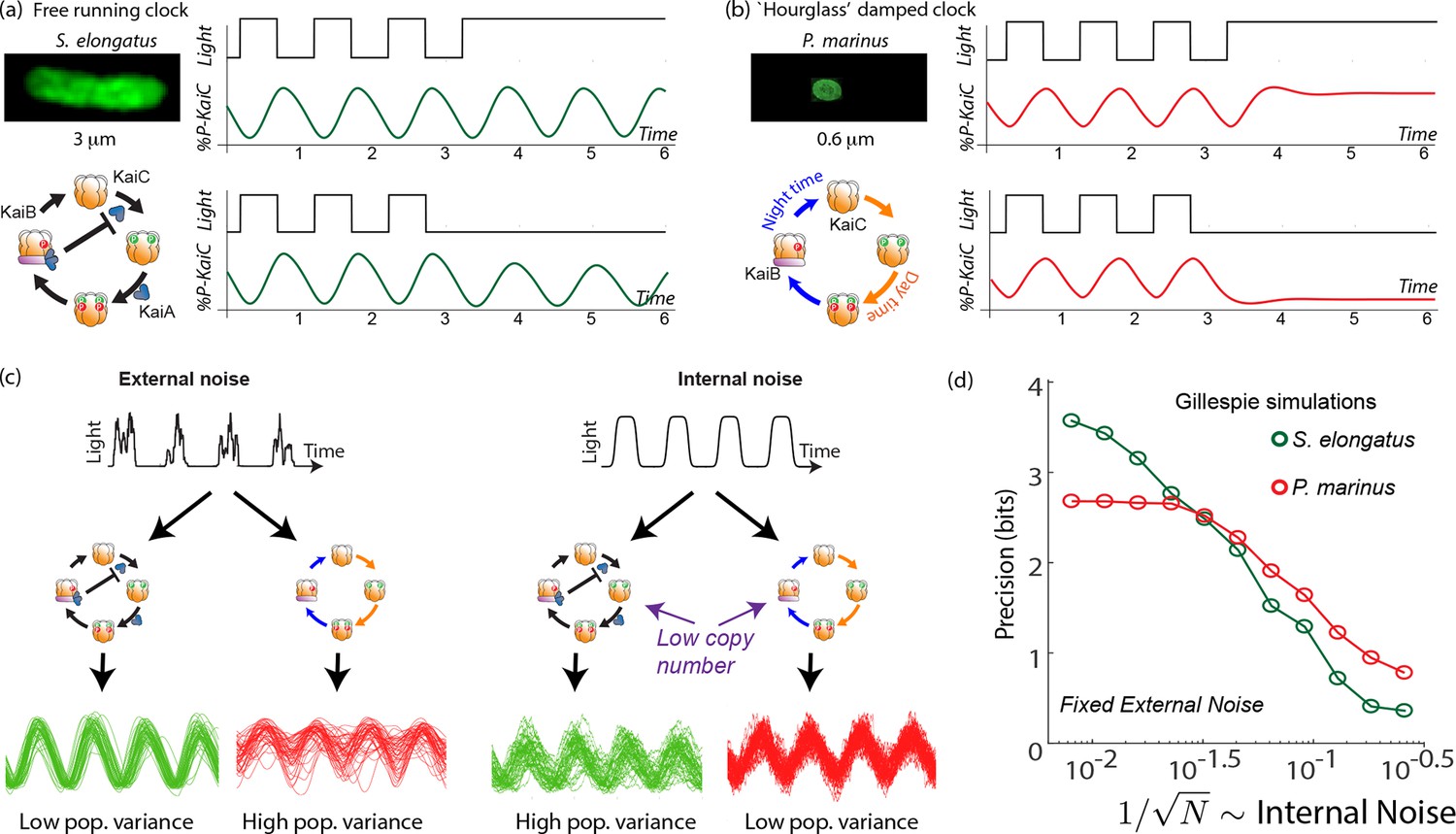
Free running clocks and damped ‘hourglass’ clocks are equally good time-keepers in noiseless conditions but internal and external fluctuations reveal significant differences.
(a) Free running circadian clocks, such as the KaiABC protein clock in S. elongatus, show rhythms in both oscillating and constant light (top) or dark (bottom) conditions. (b) In contrast, damped circadian clocks, such as that in P. marinus which lacks Kai A, show rhythms only in changing light conditions and decay to a fixed state in constant conditions. (c) When subject to external noise (i.e., weather-related amplitude fluctuations in light), simulations of the free running clock show low population variance while the damped clock shows high variance. In contrast, Gillespie simulations with high internal noise due to low copy number of Kai molecule reveals that damped clocks are much more robust than free running clocks. (d) A systematic study of clock precision (i.e., mutual information between clock state and time) at fixed external noise but decreasing Kai protein copy number reveals that free running clocks are preferred at low internal noise but damped clocks are preferable at sufficiently high internal noise.
Figure 2
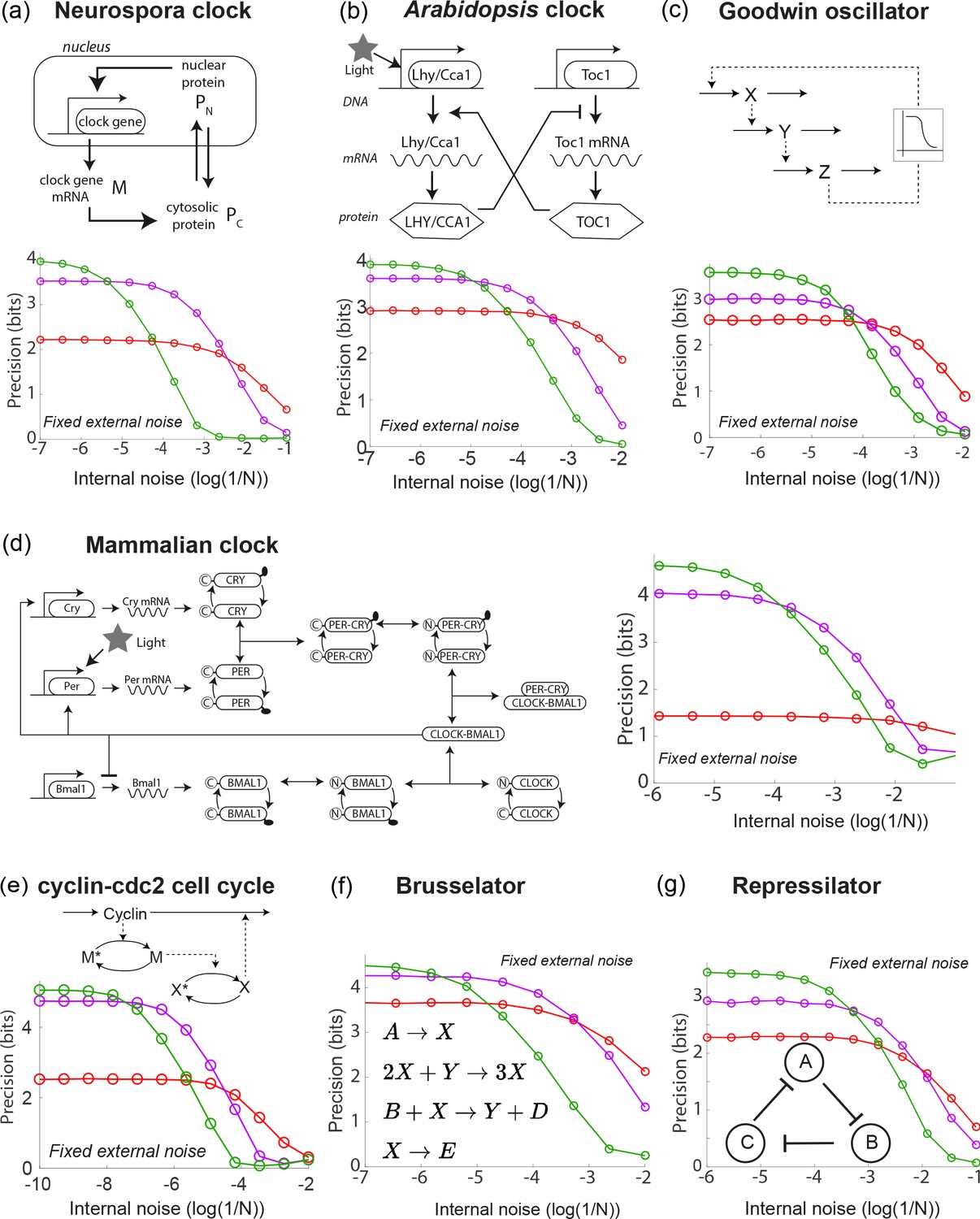
A diverse range of biochemical oscillators show the trade-off between resistance to external and internal noise.
For each oscillator, the regime (green) of largest free running amplitude relative to the driving strength is most robust to external fluctuations but is most fragile to internal noise. In contrast, damped oscillations (red) are robust to internal noise and thus preferable at sufficiently high internal noise. Regimes (purple) of intermediate free running amplitude are preferred at intermediate internal noise levels. (a–g) Diverse biochemical oscillators from the literature were simulated with increasing internal noise while driven by a periodic square wave light signal with fixed strength external noise, using the external coupling and parameters specified in the original publications (Leloup et al., 1999; Schmal et al., 2014; Locke et al., 2005; Leloup and Goldbeter, 2003; Goldbeter, 1991; Goodwin, 1965; Gonze and Abou-Jaoudé, 2013; Kondepudi and Prigogine, 2014; Elowitz and Leibler, 2000; Buşe et al., 2009). Clock precision is defined as mutual information between outputs and time. The original publications identified a Hopf bifurcation parameter in these models, with free running oscillations on one side and damped oscillations on the other. Green and purple data correspond to parameter regimes with large and smaller amplitude free running oscillations relative to driving amplitude while the red data corresponds to a damped oscillator. Details in Appendix 2.
Figure 3
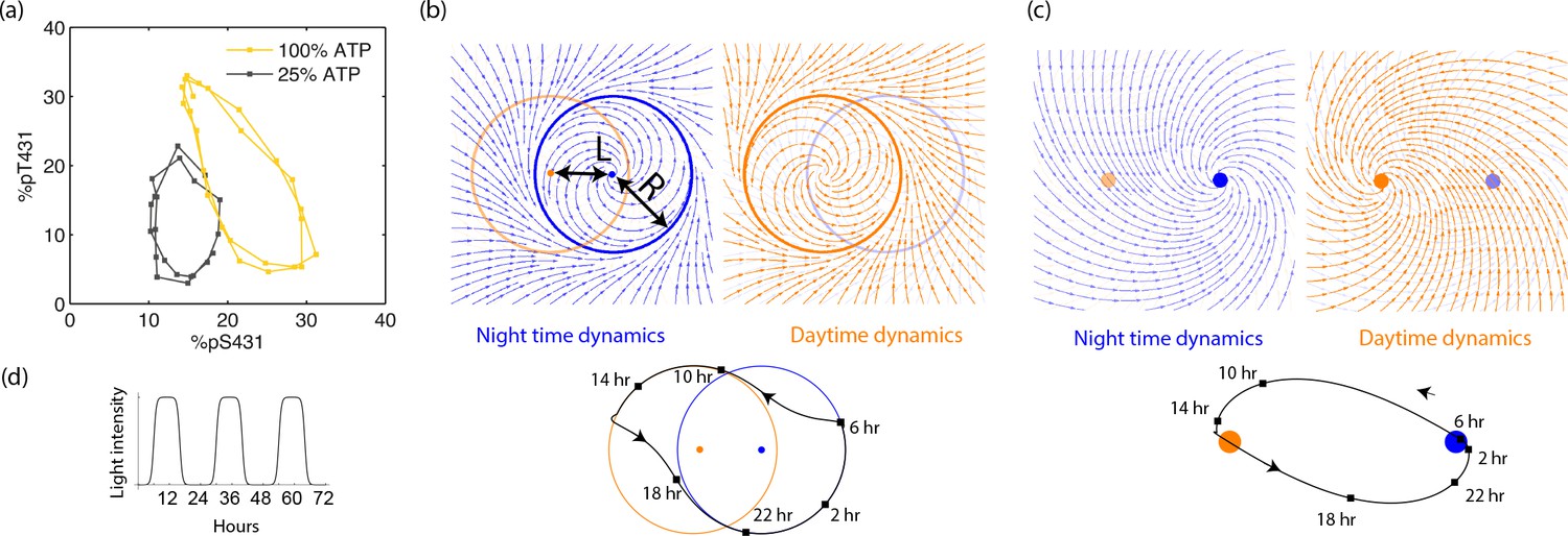
Experiments and models of biological clocks show that external driving can be viewed as a switch between distinct day-time and night-time dynamics.
(a) Experiments on the Kai system at distinct ATP levels corresponding to day and night conditions reveal limit cycles shifted relative to each other in a phosphorylation space for Kai (reproduced from [Leypunskiy et al., 2017[). Similar behavior (Winfree, 2001) is seen in models of diverse biochemical oscillators studied in Figure 2. (b) We build a minimal model of such driven clocks as a limit cycle of radius whose center is shifted by a distance between day and night. In cycling conditions (see signal in (d)), an entrained clock’s state executes a trajectory that encompasses both limit cycles as shown (bottom). (c) For damped clocks (Saunders, 2002), phenomenology suggests that the day and night limit cycle dynamics are replaced by a point attractor whose position changes between day and night. The relaxation time between the day and night attractors is comparable to hours, giving rise to the trajectory shown in cycling conditions. (d) The plot shows cycling conditions of light intensities that couple to (b) and (c).
Figure 4
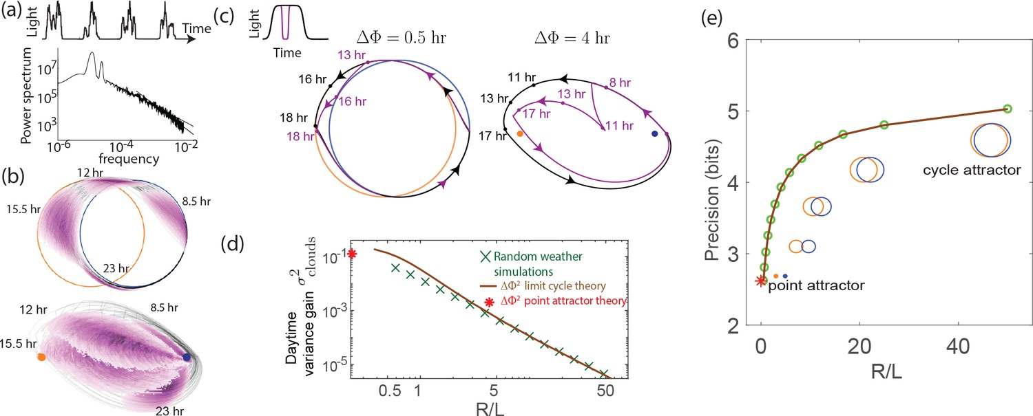
External weather-related light fluctuations are filtered out by limit cycle attractors but not by point attractors.
(a) Light intensity levels fluctuate on a range of time scales due to weather (power spectrum reproduced from Gu et al., 2001). (b) A population of limit cycle clocks of identical fixed geometry, subject to different realizations of weather conditions, show non-overlapping distributions (purple blobs) at different times of the day. Point attractor clocks form larger and more overlapping distributions. (c) A single representative dark pulse of duration causes only a min phase lag in limit cycles since the trajectory’s deviation (purple) is fundamentally bounded by the circular attractor. In contrast, hr for the point attractor since the trajectory is in free-fall towards the blue night-time attractor. (d) The geometrically computed phase shift for a dark pulse of any fixed duration and time of occurrence (see Appendix 5) drops rapidly as for large- limit cycles; this theoretical prediction agrees well with the population variance gain over a day in simulations. (e) Consequently, weakly driven limit cycles (i.e., high ) can tell time with high precision.
Figure 5
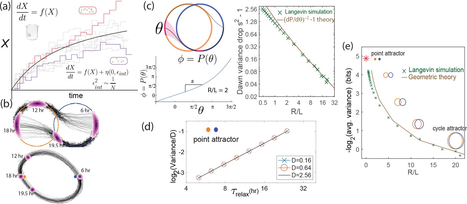
Internal fluctuations severely affect continuous attractors but not point attractors.
(a) We model fluctuations due to finite copy number as Langevin noise with mean zero and standard deviation , resulting in a diffusion constant for the clock state. (b) The flat direction of limit cycles cannot contain diffusion, leading to large increases in population variance of clock state during each day (and night). In contrast, point attractor dynamics have constant curvature at all times, leading to a constant population variance over time. (c) The variance drops at dawn and dusk for limit cycles during the off-attractor dynamics between the day and night cycles. As with external noise, the variance drop is predicted by the slope of the circle map between the cycles. This dawn/dusk drop goes to zero for large limit cycles but variance still increases during the day and night. (d) The variance for point attractors is , a constant determined by the curvature of the harmonic potential. (e) Thus, with only internal noise present, the precision of limit cycle clocks increases with increasing separation , asymptotically approaching the performance of point attractors.
Figure 6
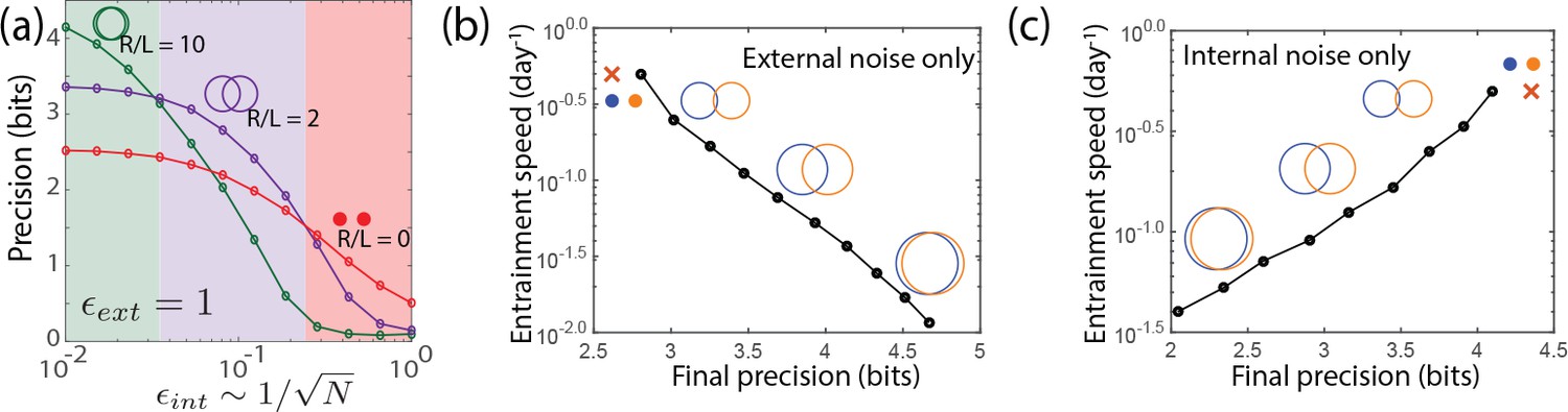
Large- limit cycle attractors, which correspond to large amplitude free running clocks, outperform all other oscillators in projecting out external noise but are least robust to internal noise.
(a) Point attractors and smaller limit cycles (red and purple curves) show low precision (i.e., low mutual information) but do not degrade as much as large- limit cycles with increasing internal noise . Thus this simple dynamical systems model of clocks reproduces and explains the trade-off seen in the complex biochemical clocks shown in Figures 1 and 2. (b,c) Speed-precision trade-off. (b) With external noise alone, the most precise clocks (i.e., large limit cycles) average over longer signal history and are thus the slowest to entrain, that is, slow to transform a population with uniform phase distribution to the steady state distribution. (c) However, with internal noise alone, there is no trade-off between speed and precision; faster entraining clocks (i.e., point attractors) are more accurate since slow clocks are exposed to more internal noise.
Appendix 1—figure 1
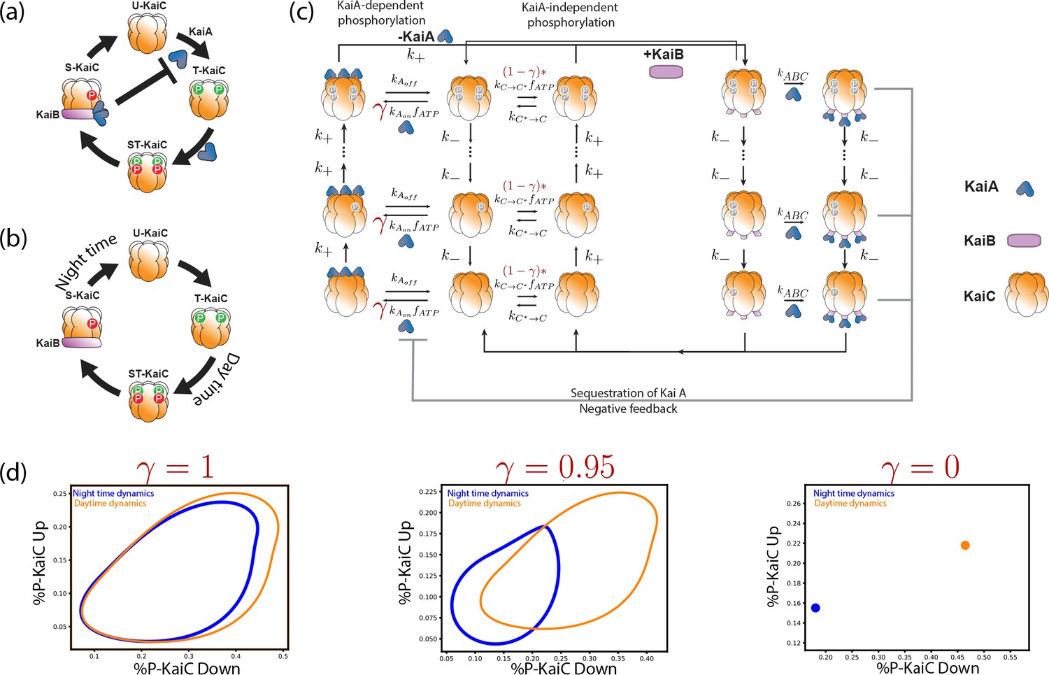
Explicit biochemical KaiABC model simulated using the Gillespie algorithm.
(a) The experimentally well-characterized clock in S. elongatus consists of a negative feedback-enabled self-sustained oscillator. KaiBC complexes sequester KaiA, preventing runaway KaiC molecules from going through the cycle independently. (b) The genome of P. marinus lacks kaiA. We assume a minimal model consistent with known facts (Rust et al., 2007) about this clock; KaiC phosphorylation proceeds without KaiA and hence different KaiC hexamers can proceed independently through the cycle. (c) We combine both clocks in one model with an interpolating parameter that selects between an S. elongatus-like KaiA-dependent pathway and an P. marinus-like KaiA-independent pathway. All reactions shown are assumed to be first order mass-action kinetics. We simulate such a system at different overall copy numbers using the Gillespie algorithm. (d) We find limit cycles for . The resulting limit cycles for violate the simplifying assumptions used in our dynamical systems (e.g., non-circular cycles of different size); and yet our results are qualitatively validated by this model (Figure 1d from the main text).
Appendix 4—figure 1
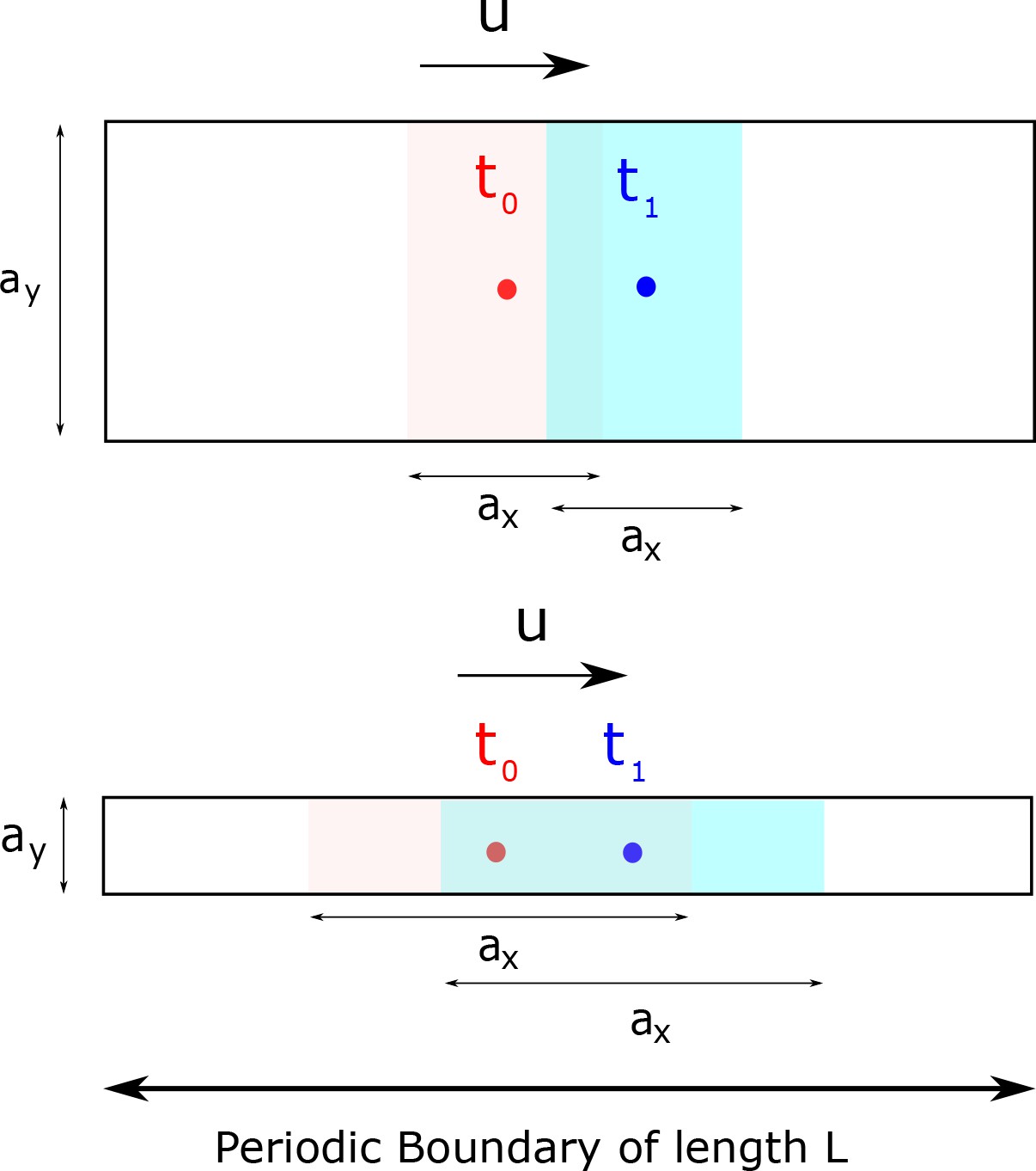
Mutual information between clock state and time is only affected by the variance of the clock state distribution at a given time along the direction of motion and not orthogonal to it.
In this toy example, we assume the distribution to be supported on a rectangle of size and in a 2d clock state space. The clock state moves at a speed in the x-direction. Time telling quality is affected by how much the population at different times overlap with each other. Consequently, clocks with large and small (bottom) have lower mutual information relative to clocks with small and large (top). Consequently, we use the population variance along the direction of motion as an instantaneous measure of time-telling ability in the paper.
Appendix 5—figure 1
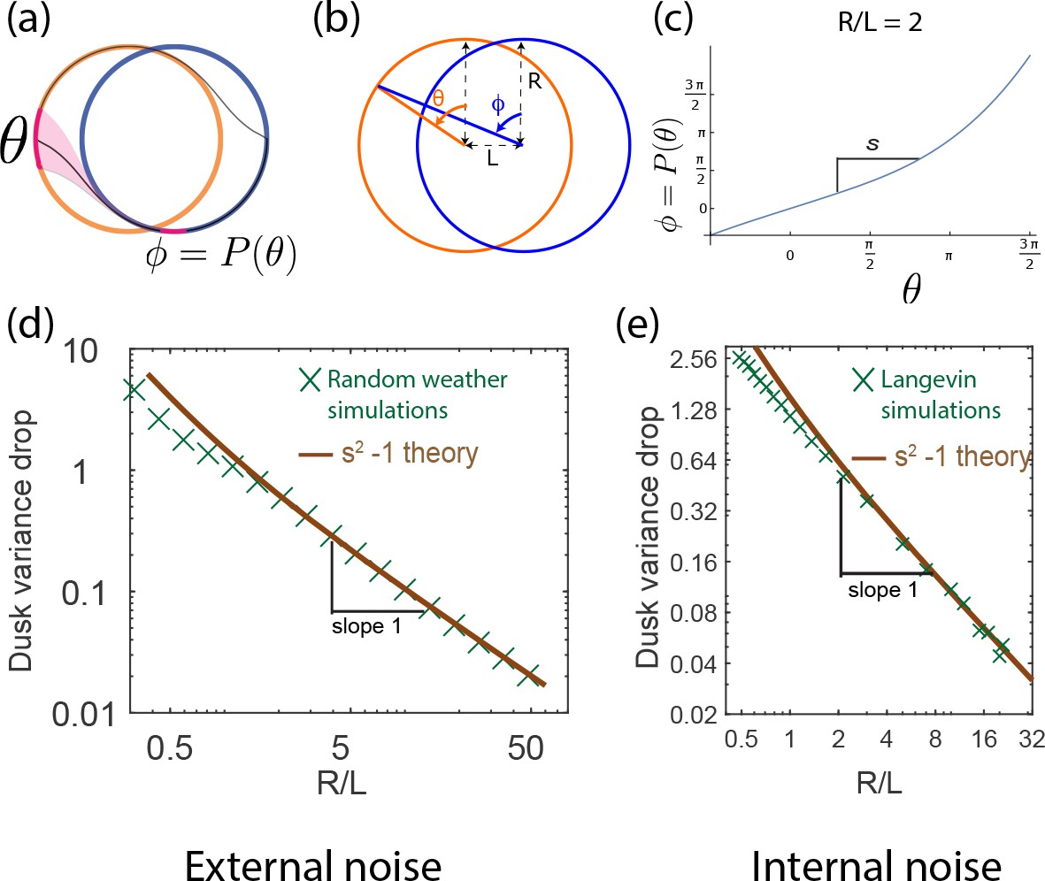
The population variance of clock states is reduced by dusk and can be computed geometrically.
(a) A population of clocks near state on the day cycle is mapped to the neighborhood of state on the night cycle by the dusk transition. We define to be the map relating the clock state on the day cycle just before dusk to its eventual position on the night cycle after dusk (assumed greater than the relaxation time). (b) This map can be analytically computed for circles of size R with centers separated by length L. (c) For a given R/L = 2 , we obtain shown here. Since corresponds to the dusk time of the entrained trajectory, the slope at determines the change in population variance of clock states at dusk. (d,e) The variance drop at dusk, defined as at dusk, seen in both the external (averaging over weather) and internal noise (averaging over Langevin noise) simulations agree well with the geometrically computed , especially at large . We find that for large- limit cycles.
Appendix 5—figure 2
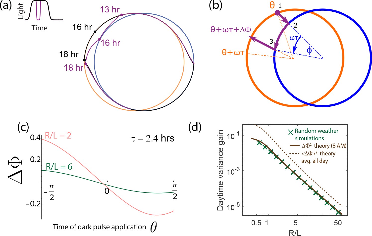
Increase in population variance due to random weather conditions can be estimated from the phase shifts due to dark pulses (i.e., the Phase Response Curve).
(a) A single dark pulse administered during the day shifts the phase of a clock (purple) relative to a clock that experiences no such dark pulse (black). (b) We can compute the phase shift due to such a dark pulse geometrically by computing the deviation in trajectory. Assuming a dark pulse of length , the clock evolves for a time according to the night cycle dynamics. At the end of such a pulse, we switch back to the day limit cycle and compute the resulting phase shift . (c) The resulting phase shift due to a pulse of length hrs, depends on the time when it is administered but is generally smaller for larger . (d) We find that for a specific hrs dark pulse administered at the same time (8 AM) falls as for large- limit cycles. This trend matches the variance gain seen in stochastic simulations that average over random weather conditions (pulses of different length, intensity and time of application). The broken brown curve shows a theoretical prediction for such an average , obtained by sampling the curve shown in (c) at different points of application and differing intensity. Despite the presence of a variance-reducing zero around mid-day in (c), drops as , much as for any particular pulse. (Brown theory curves translated together using one fitting parameter).
Additional files
-
Transparent reporting form
- https://doi.org/10.7554/eLife.37624.009
Download links
A two-part list of links to download the article, or parts of the article, in various formats.
Downloads (link to download the article as PDF)
Open citations (links to open the citations from this article in various online reference manager services)
Cite this article (links to download the citations from this article in formats compatible with various reference manager tools)
Biophysical clocks face a trade-off between internal and external noise resistance
eLife 7:e37624.
https://doi.org/10.7554/eLife.37624


