Conditioning sharpens the spatial representation of rewarded stimuli in mouse primary visual cortex
- University of Amsterdam, Netherlands
Figures
Figure 1 with 3 supplements
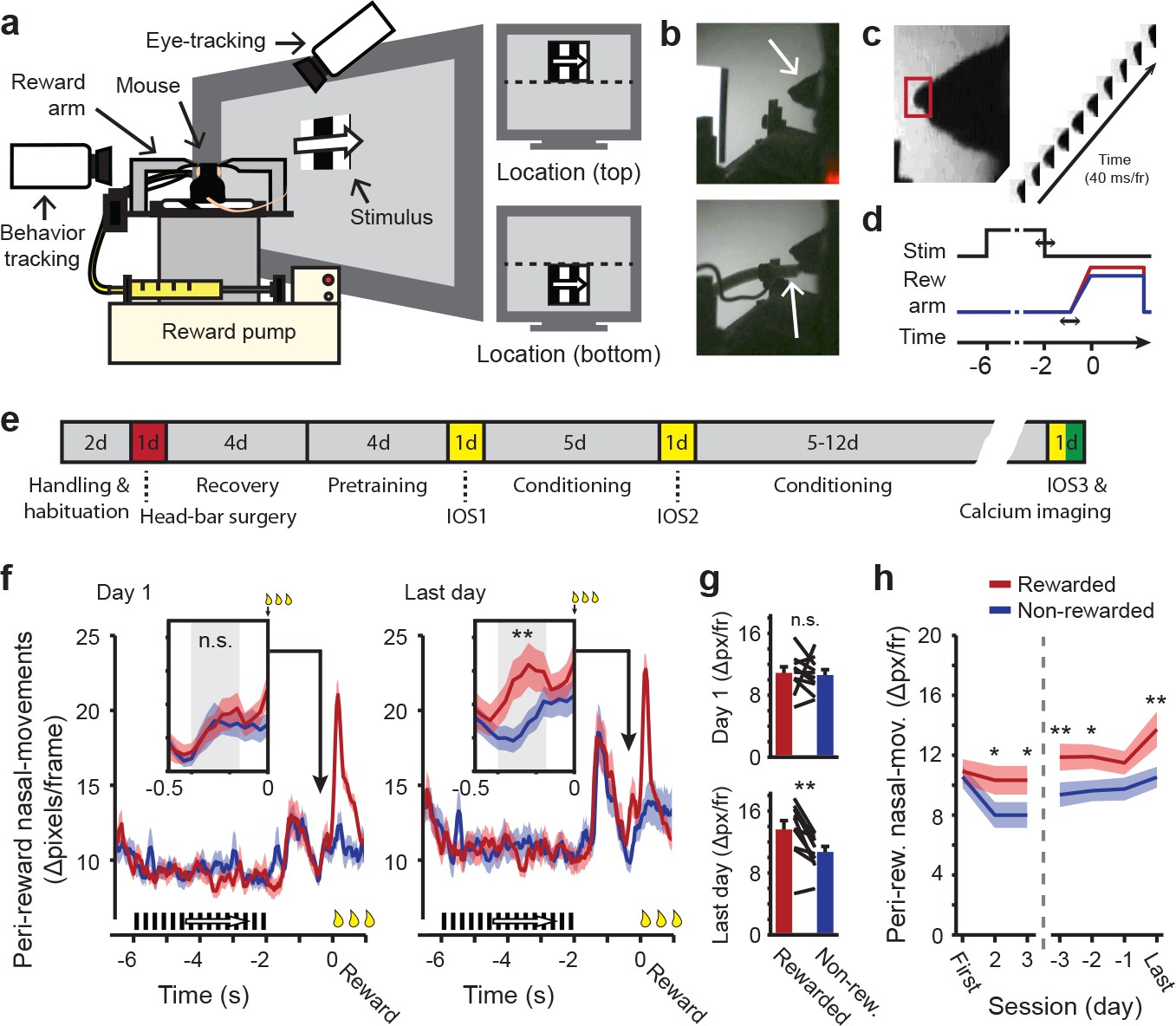
Classical conditioning in head-restrained mice.
(a) Schematic depiction of the setup used for classical conditioning. Head-restrained mice faced a computer screen at a 45° angle. Reward (Vanilla dessert) was delivered through a tube on a movable arm (Reward arm). Cameras recorded putative sniffs and licks (Behavior tracking) and eye movements (Eye-tracking). Right: Example of compound stimuli used for conditioning; location (‘top’ or ‘bottom’) predicted reward, orientation of drifting gratings was identical in both locations during conditioning. (b) Outline of the mouse head (arrow, top panel). Reward-delivery (arrow, bottom panel). (c) Example of putative sniff, video-tracked in a small area surrounding the tip of the nose (red box). (d) Schematic showing the sequence of events in a single conditioning trial. Upper line shows stimulus onset and offset. Middle line represents reward arm position for rewarded (red) and non-rewarded (blue) trials. Lower line indicates time. Horizontal arrows indicate jitter in timing. (e) Timeline of the full conditioning experiment in days (‘#d’ indicates number of days; IOS1, IOS2 and IOS3 indicate intrinsic optical imaging time points; Red indicates day of head-bar implantation; Green indicates day of calcium imaging). (f) Peri-reward nasal movements in the first (left panel) and last (right panel) conditioning session. A large peak in nasal movements can be seen during reward delivery (t = 0) and in response to stimulus offset, 1.5 s before (non) reward. Reward-arm movement started at −0.4 s in both rewarded and non-rewarded trials. Insets: Nasal movements in the anticipatory period, when the arm was en-route, but did not exceed the non-reward position (gray box, −0.4 to −0.16 s before reward time). (g) Mean nasal movement in the anticipatory period in the first (top panel) and last (bottom panel) conditioning session. Single lines represent individual mice. (h) Mean anticipatory nasal movements on different days of the conditioning experiment. All panels: Data represent mean ± SEM across mice. Red lines: rewarded trials. Blue lines: non-rewarded trials. *p<0.05, **p<0.01, WMPSR test.
Figure 1—figure supplement 1
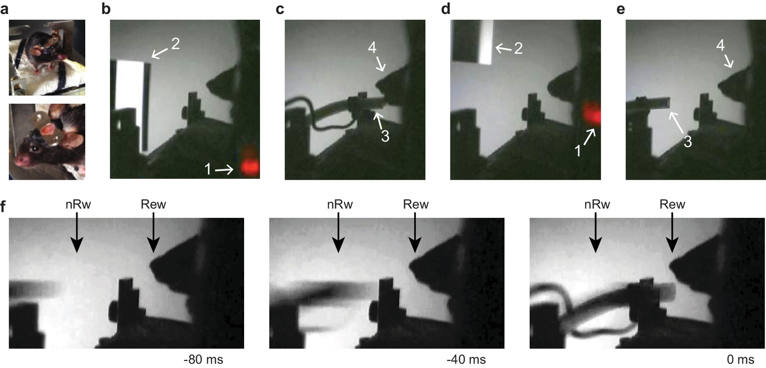
Operational procedures of the experimental apparatus for head-restrained conditioning.
(a) Top panel: Pre-training and handling of a mouse that was implanted with a chronic head bar. Syringe contained liquid reward (Vanilla desert, see Materials and methods). Bottom panel: Zoom in on stainless steel head fixation plate. (b–e) Video monitoring of task-related mouse behavior in rewarded (b–c) and non-rewarded (d–e) trials. (1) Trial onset light (only visible to experimenter); (2) Rewarded or Non-rewarded stimulus; (3) Reward tube in reward or non-reward position; (4) Silhouette of mouse head. (f) Timing of arm movement in rewarded and non-rewarded trials with 40 ms (single video frame) resolution. 'Rew' indicates reward position endpoint, 'nRw' indicates non-reward endpoint of the arm. Left image: Neither position is reached. Middle image: Non-reward position reached. Right image: Reward position reached.
Figure 1—figure supplement 2

Peri-reward oral-movement during visual conditioning.
(a) Example of a putative lick. Licks were detected in the area, delineated by the position of the lower and upper jaw during visually identified licks (red box; manually outlined per video). (b) Peri-reward oral movement (putative licks) in the first conditioning session. A large peak in oral movement indicates reward consumption at the time of reward delivery (t = 0). The inset displays putative licks from −0.5 to 0 s before reward, with the gray region indicating the anticipatory period from −0.4 to −0.16 s before the arm reached the reward position. Red: Rewarded trials; Blue: non-rewarded trials. (c) Same as b) but for the last conditioning session of each mouse. Pre-reward oral-movement was stronger in the anticipatory period of rewarded trials compared to non-rewarded trials (**p<0.01, WMPSR test). (d) Mean oral movement in the anticipatory period of the first training session. Single lines represent individual mice. (e) Mean oral-movement in the anticipatory period of the last conditioning session. All but one animal showed more intense anticipatory oral-movement in rewarded trials compared to non-rewarded trials (**p<0.01, WMPSR test). (f) Difference in oral-movement during the first three and last four conditioning sessions (*p<0.05, **p<0.01; WMPSR test). All data are presented as mean ± SEM across mice.
Figure 1—figure supplement 3
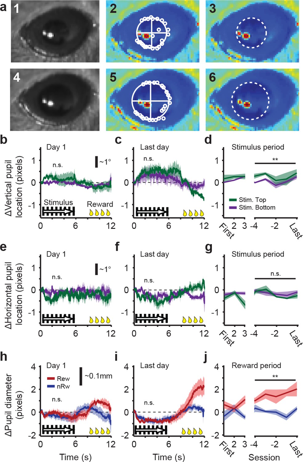
Tracking of pupil diameter and movement during head-restrained conditioning of awake mice.
(a) Example of pupil detection in a single video frame (acquired using a NIR camera) of a mouse eye with an average sized (1) and large sized (4) pupil. The center of the pupil was approximated using a radial symmetry transform (see Materials and methods). From this point outwards, the edge of the pupil was estimated towards all directions (white circles in 2 and 5), except for the direction of the reflection spot (similar to the Starburst algorithm; see Materials and methods). A circular fit (straight lines in 2 and 5) provided the center and diameter of the pupil (3 and 6). (b) Tracking of vertical pupil center in visual conditioning trials of the first training session. Units are in pixels, which correspond roughly to ~2 retinal degrees (see scale bar). Green traces show data from trials with a stimulus in the upper part of the visual field ('Stim. Top') and purple traces are for stimuli in the lower part of the visual field ('Stim. Bottom'; differences were n.s.). Black/white bars from 0 s to 6 s mark visual stimulation. Yellow drops plotted from 8 s to 12 s mark reward period. (c) Idem, but for the last training session. (d) Average vertical pupil movement during the 6 s stimulus period in the first three and last four conditioning sessions (**p<0.01, Mann-Whitney U test across four time points). (e,f,g) Same as in (b), (c) and (d), but for horizontal pupil movement. (h) Pupil diameter in the first training session for trials in which the rewarded stimulus (red) was shown, versus trials in which the non-rewarded stimulus (blue) was shown. (i) Same as h), but for the last day of conditioning. (j) Average pupil dilation during the last 2 s of reward consumption in the first three and last four conditioning sessions (**p<0.01, Mann-Whitney U test across four time points). All data in b) to j) are relative to baseline and presented as average ± SEM across six mice.
Figure 2 with 1 supplement
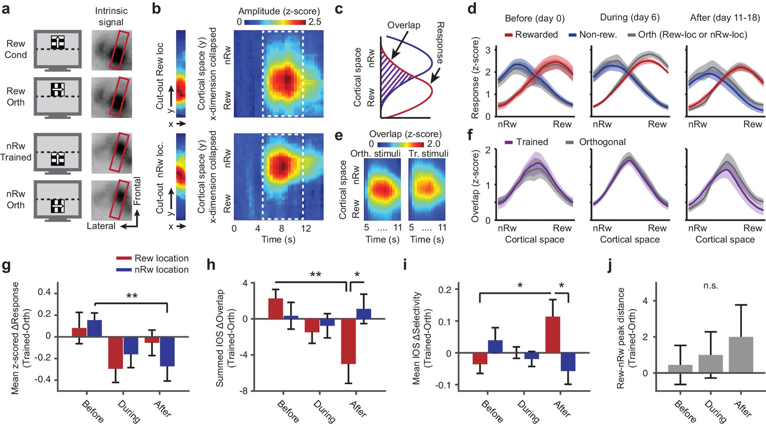
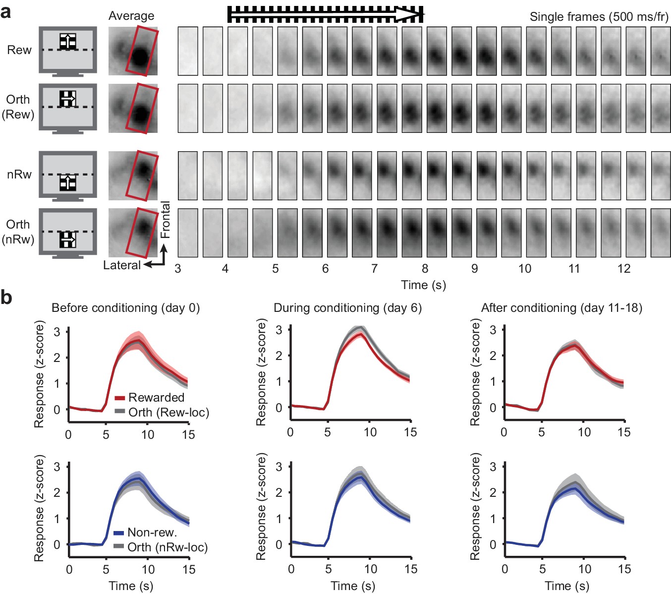
Repeated imaging of intrinsic optical signals in V1 of mice subjected to conditioning.
(a) Visual stimuli (left panels) and average stimulus-induced intrinsic optical signal (IOS; right panels), showing strong retinotopically selective responses to the rewarded and non-rewarded location in area V1 (within red boundary) and weaker responses in the lateral supplementary visual areas LM and AL (to left of red box). Orth, orientation orthogonal to trained orientation (Cond). (b) Left panels: Example of 11-pixel wide cutout from the red box in a, that was automatically rotated so as to include the cortical area of maximal activation for both the top and bottom stimulus location. Right panels: The IOS response to each stimulus as a function of cortical space (maximally separating the top and bottom stimulus) and time (derived from the 11-pixel wide cutouts by collapsing the ‘x’ dimension per imaging frame and concatenating time points). Upper panels: Response to rewarded location and orientation. Lower panels: Response to non-rewarded location and orientation. (c) Schematic showing quantification of the response amplitude and overlap of cortical responses to visual stimuli in adjacent retinotopic locations. (d) Mean ± SEM z-scored amplitude of the IOS response (across the period of maximum activation, 7 to 11 s) as a function of cortical space along the axis that maximally separates the rewarded and non-rewarded stimulus. Red: Rewarded stimulus; Blue: Non-rewarded, trained stimulus; Grey: Orthogonal orientations at the rewarded or non-rewarded location respectively. Left panel: Data acquired before the first conditioning session (day 0; IOS1, see also Figure 1e). Middle panel: After five conditioning sessions (IOS2). Right panel: Data acquired after the last conditioning session on the same day as, but before, calcium imaging (IOS3). (e) Mean overlap (across all mice) between the response to the orthogonal or trained stimuli in the rewarded and non-rewarded locations as a function of cortical space (y-axis) and time (x-axis). Scale bar above applies for both panels. (f) As in d), but for the overlap between the response to the rewarded and non-rewarded trained stimulus (plotted in Violet). (g) ΔResponse amplitude (difference between trained and control orientations) in the cortical region that responded to the rewarded location (red) and non-rewarded location (blue) separately, across imaging time points (**p=0.0039, Kruskal-Wallis, post hoc WPMSR test). (h) As in g), but for ΔOverlap per region and across imaging time points (*p=0.039, WMPSR test; **p=0.011, Kruskal-Wallis test, post hoc WMPSR test). (i) As in g), but for ΔSpatial selectivity (Rewarded vs. Non-rewarded: *p=0.039, WMPSR test; Before vs. After: *p=0.046, Kruskal-Wallis test). (j) Distance between the peak responses to the spatially segregated stimuli (difference between trained and orthogonal control stimuli, positive values indicate larger distance between trained stimulus representation peaks).
Figure 2—figure supplement 1
Repeated intrinsic optical signal imaging in V1 of a mouse subjected to conditioning.
(a) Example data of mouse #15. Left panels: Visual stimuli used for this mouse. Middle panels: Average stimulus-induced intrinsic optical signal (IOS), showing retinotopically selective responses to the rewarded (Rew) and non-rewarded (nRw) location in area V1 (within red boundary), but also in the lateral supplementary visual area LM (situated left of the red box). Right panels: Single image frames (2 Hz sampling rate) from a single trial for each stimulus. On top, black bars and arrow above indicate time of stimulus presentation. (b) Intrinsic signal imaging data across nine mice. Mean ± SEM amplitude of the inverted z-scored IOS response to each of the stimuli, plotted against time. Stimulus onset is at t = 4 s. Red: Rewarded stimulus; Blue: Non-rewarded stimulus; Grey: Orthogonal orientations at the rewarded or non-rewarded location respectively. Left column: Data acquired before the first conditioning session (day 0; IOS1). Middle column: After five conditioning sessions (IOS2). Right column: Data acquired after the last conditioning session on the same day as, but before, calcium imaging (IOS3).
Figure 3 with 1 supplement
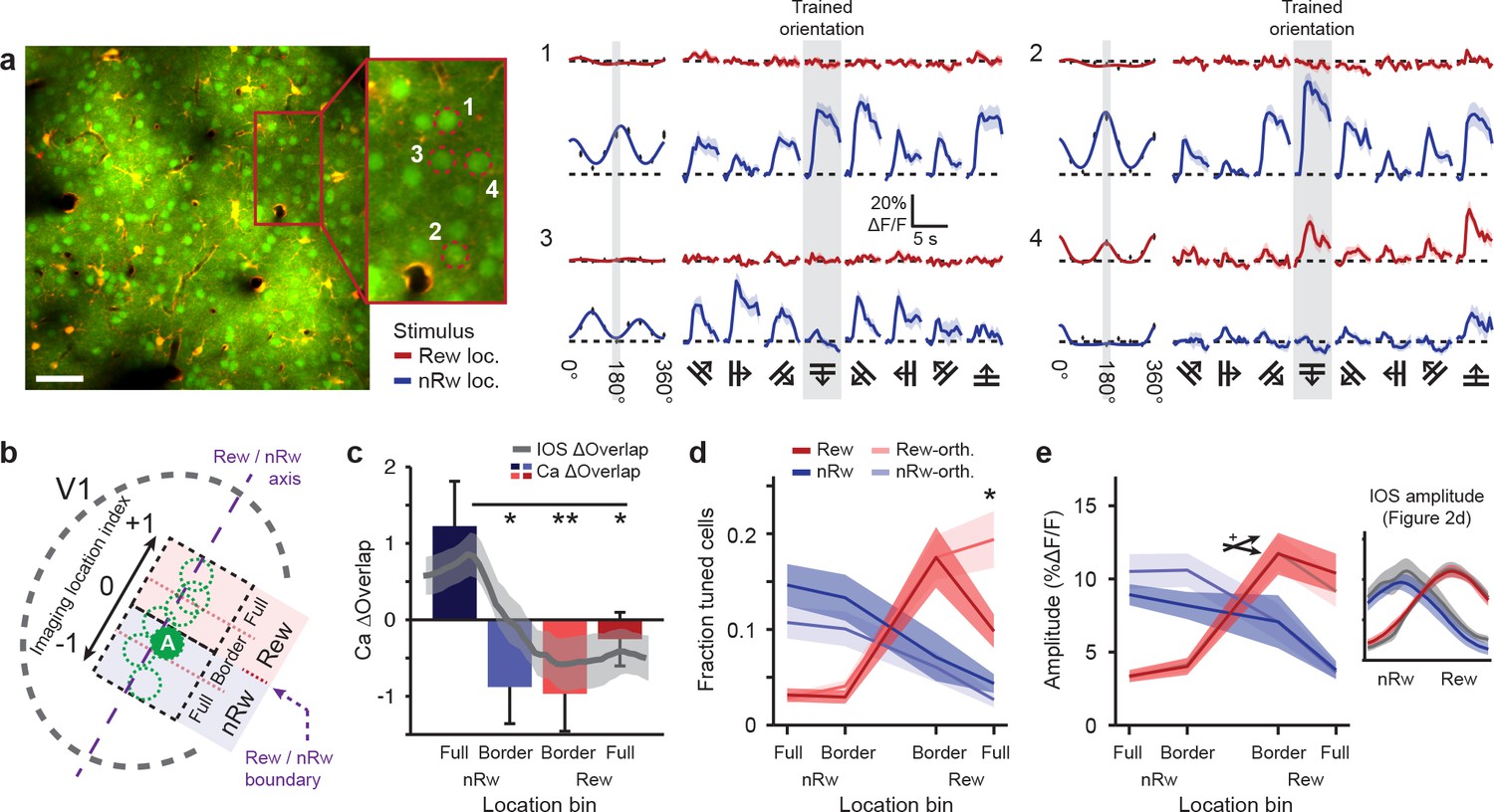
Two-photon imaging of orientation-tuned responses in different retinotopic regions of V1.
(a) Example of calcium imaging in a field of view that was located in the Border non-rewarded region. Left: Overview image and inset showing neurons loaded with the calcium indicator OGB1-AM (green) and double-labeled astrocytes (yellow). Right panels 1–4 correspond to ROI’s 1–4 in inset a. Left columns of all 4 ROI response panels: Fitted tuning curves for movement orientation/direction (Red: visual stimulus in rewarded visual field; Blue: visual stimulus in non-rewarded visual field) and mean (±SEM) response to each of the eight directions (black vertical bars). Traces on right: Average ∆F/F time courses for each of the eight movement directions separately (Grey shaded columns: trained orientation). (b) Top-view scheme of the imaging locations on the visual cortex. The dashed purple line represents the ‘rewarded/non-rewarded axis’. The boundary between the rewarded and non-rewarded stimulus representations is at location index value ‘0’ and marked with a dashed purple arrow (see Online Materials and methods). ‘A’ indicates the approximate location of the field of view in a. (c) Calcium-imaging derived ∆Overlap in each of the location bins. Overlaid gray line represents mean (±SEM, shaded region) of the overlap measured after conditioning using intrinsic imaging (*p<0.05, **p<0.01, Kruskal-Wallis, post-hoc Mann-Whitney U test). This overlap was computed as in Figure 2. (d) Fraction of orientation-tuned neurons preferring the rewarded (red), non-rewarded (blue) or orthogonal (lighter shaded colors) stimuli (*p<0.05, Anova, post-hoc t-test). (e) Average response amplitude in ∆F/F (%) of significantly orientation-tuned neurons to their respective preferred orientations, per location bin. Red: Cells preferring the rewarded orientation. Light red: Cells preferring the orthogonal stimulus in the rewarded location. Blue and light blue: The same, but for the non-rewarded stimulus location. Crossed arrow indicates Anova interaction effect,+P < 0.05. Inset on the right shows the mean (±SEM) response amplitude as measured in the last intrinsic imaging session (see Figure 2d).
Figure 3—figure supplement 1
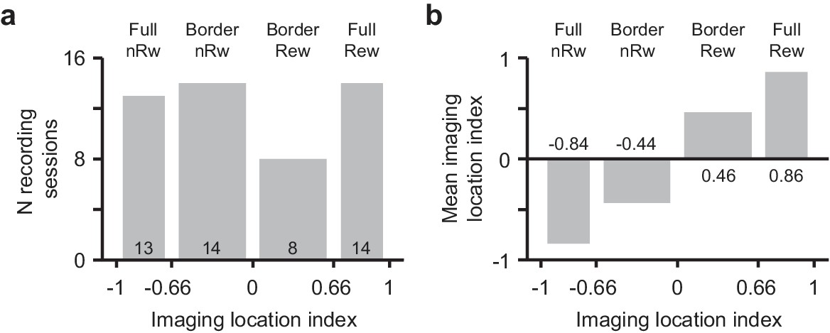
Binning of recording location into discrete groups.
(a) Histogram of the number of recording sessions with an imaging location index (see Online Materials and methods for details) ranging from −1 (Non-rewarded side, nRw) to +1 (Rewarded side, Rew), classified as ‘Full non-rewarded’, ‘Border non-rewarded’, ‘Border rewarded', ‘Full rewarded’. The width of the bar is indicative of the range of included session location indices. (b) Mean imaging location index in each of the location bins showing a linear increase of location selectivity.
Figure 4 with 1 supplement
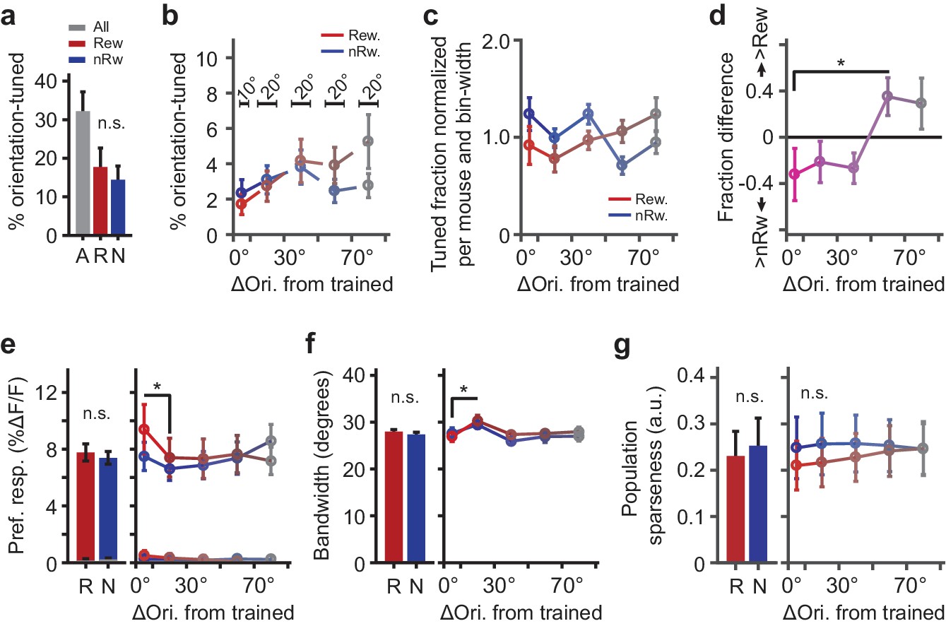
Parameters describing orientation-tuned neurons preferring the rewarded or non-rewarded stimulus location.
(a) Left panel: Mean ± SEM percentage of significantly orientation-tuned cells per mouse. ‘A’: All locations. ‘R’: Rewarded location. ‘N’: Non-rewarded location. (b) Absolute fraction of orientation-tuned neurons responding to the rewarded (red) and non-rewarded (blue) location separately, and relative to the trained orientation (e.g. neurons with a preferred orientation nearly identical to the trained orientation were in bin 0°−10°). Bars above data points indicate relative bin-widths. Note that because the left-most bin (0–10 degrees) is only half the width of the other bins, it is expected to contain half of the fraction of the other bins. (c) Distribution (normalized per mouse and bin-width) of preferred orientations relative to the trained orientation (given a flat distribution of preferred orientations, the expected fraction of each bin would be 1.0). (d) Difference in fraction of orientation tuned neurons to the rewarded minus the non-rewarded location (positive values indicate a larger fraction of neurons tuned to the rewarded stimulus location; *p=0.042, Kruskal-Wallis test, post hoc WMPSR test). (e) The mean (±SEM) ∆F/F response to the preferred direction as a function of the preferred orientation relative to the trained orientation for rewarded and non-rewarded location-tuned neurons separately (*p<0.05, WMPSR test). The lines that fall between 0% to 0.5% ∆F/F show the response amplitude of the same neurons, but to the orientation that was orthogonal to the preferred orientation. We note that the sequence of bins is thus not representative of the entire tuning curve but shows the response amplitude to a specific (preferred or orthogonal) direction. (f) Same as e), but for bandwidth (*p<0.05, WMPSR test). (g) As in e), but for sparseness of the tuning curve response calculated across the population all neurons. For all panels: Red colors indicate groups of cells preferring ‘rewarded’ conditioned orientations, while blue colors indicate groups of cells preferring ‘non-rewarded’ trained orientations. Both colors fade to gray, indicating that the preferred orientation of the cells becomes more dissimilar from the trained orientation.
Figure 4—figure supplement 1
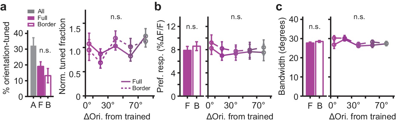
Comparison of orientation tuning parameters between cells located close and far away from the rewarded/non-rewarded border.
(a) Distribution of preferred orientation of orientation-tuned neurons relative to the trained orientation (mean per bin, averaged ± SEM across mice). 'A': All locations. 'F': Full imaging regions. 'B': Border imaging regions. (b) The mean (±SEM, averaged across mice) ∆F/F response to the preferred direction as a function of the preferred orientation relative to the trained orientation. (c) Idem, but for the tuning curve bandwidth. For all panels, solid lines: Data from the Full rewarded and Full non-rewarded regions of the visual cortex. Dashed lines: Data from the Border rewarded and Border non-rewarded regions of the visual cortex. All performed tests compared data from Full and Border regions across mice, no significant differences were observed.
Figure 5

Population coding of visual field location by visual cortex neurons.
(a) Left panel: Performance of decoding retinotopic location using activity of simultaneously recorded neurons in regions close to the rewarded/non-rewarded location border as a function of increasing population size. Chance level is 50%. Inset illustrates which field-of-view locations were included in these data. Dark purple curves are data from the population with a preferred orientation similar to the trained orientation. Light purple curves are data from neurons preferring orientations differing 45° from the trained orientation. Gray curves are for the data from cells preferring orientations orthogonal to the trained orientation. Data are shown as mean ± SEM averaged across 9 mice. **p<0.01, WMPSR test. Right panel: Same, but for neurons recorded in regions further away from the rewarded/non-rewarded location border. (b) Per mouse, the mean conditioning related-improvement in coding for visual field location was plotted against the behavioral difference in nasal (upper panel) and oral movement (lower panel) to the rewarded (Rew) and non-rewarded (nRw) stimulus location.
Figure 6

Conditioning related interactions of signal and noise correlations.
(a) Signal- and noise correlations for pairs of simultaneously recorded neurons as a function of the difference between the preferred orientation of the neurons and the trained orientation. Left panel: Data from pairs that were located further away from the region where the rewarded and non-rewarded stimuli bordered. Right panel: As left, but from pairs located in the cortical region where the representations of the rewarded and non-rewarded stimuli bordered. Solid lines: Signal correlations. Dashed lines: Noise correlations. Data are shown as mean ± error bars that indicate 95% confidence intervals. (b) Noise correlations for the selection of simultaneously recorded pairs that exhibited the 10% highest signal correlations (solid lines) and the pairs having the 10% lowest signal correlations (dashed lines). Left panel: data from the Full rewarded and Full non-rewarded regions. Right panel: data from Border rewarded and non-rewarded regions. Data are shown as mean ± error bars that indicate 95% confidence intervals (*p<0.05, **p<0.01 multiple comparison corrected bootstrap confidence intervals).
Tables
Table 1
Overview of mice included in behavioral and imaging analyses
Each row lists the following information for the mouse that can be identified by the number in the column Mouse. Rew: Location of the rewarded stimulus. nRw: Location of the non-rewarded stimulus. Dir: Direction of the moving grating used in the conditioning paradigm. Beh-track: Data for which behavior was video-tracked and included in behavioral analysis (Figure 1 and Figure 1—figure supplement 2). # trials: Total number of trials that a mouse performed across all conditioning sessions. Eye: Data included in analysis of eye-movements (Figure 1—figure supplement 3). IOS: Data included in analysis of intrinsic optical signals (Figure 2 and Figure 2—figure supplement 1). Ca2+ Full: Data included in calcium imaging analysis, 'Full imaging locations'. Ca2+ Border: Data included in calcium imaging analysis, 'Border imaging locations'. (Figures 3–6, Figure 3—figure supplement 1, Figure 4—figure supplement 1). % tuned: Overall fraction of orientation tuned neurons per mouse.
| Mouse | Rew | nRw | Dir | Beh- track | # trials | Eye | IOS | Ca2+ Full | Ca2+ Border | % tuned |
|---|---|---|---|---|---|---|---|---|---|---|
| #02 | Bottom | Top | 180° | ∗ | ∗ | 30.9 | ||||
| #03 | Top | Bottom | 0° | ∗ | ∗ | 10.9 | ||||
| #05 | Bottom | Top | 0° | ∗ | ∗ | 68.8 | ||||
| #07 | Top | Bottom | 90° | ∗ | 613 | ∗ | ∗ | ∗ | 20.2 | |
| #08 | Top | Bottom | 270° | ∗ | 378 | ∗ | ||||
| #09 | Bottom | Top | 180° | ∗ | 640 | ∗ | ∗ | ∗ | 36.9 | |
| #10 | Bottom | Top | 180° | ∗ | 575 | ∗ | ∗ | 40.6 | ||
| #11 | Top | Bottom | 180° | ∗ | 436 | ∗ | ∗ | ∗ | ∗ | 32.8 |
| #12 | Top | Bottom | 0° | ∗ | 520 | ∗ | ∗ | ∗ | ∗ | 36.9 |
| #13 | Bottom | Top | 90° | ∗ | 595 | ∗ | ||||
| #14 | Bottom | Top | 270° | ∗ | 640 | ∗ | ∗ | ∗ | ∗ | 40.7 |
| #15 | Top | Bottom | 0° | ∗ | 520 | ∗ | ∗ | ∗ | ∗ | 40.5 |
| #16 | Bottom | Top | 0° | ∗ | 480 | ∗ | ∗ | ∗ | 7.2 | |
| Total | 10 | 6 | 9 | 11 | 9 |
Additional files
-
Transparent reporting form
- https://doi.org/10.7554/eLife.37683.015
Download links
A two-part list of links to download the article, or parts of the article, in various formats.
Downloads (link to download the article as PDF)
Open citations (links to open the citations from this article in various online reference manager services)
Cite this article (links to download the citations from this article in formats compatible with various reference manager tools)
Conditioning sharpens the spatial representation of rewarded stimuli in mouse primary visual cortex
eLife 7:e37683.
https://doi.org/10.7554/eLife.37683


