Temperature explains broad patterns of Ross River virus transmission
- Stanford University, United States
- University of Florida, United States
- Emerging Pathogens Institute, University of Florida, United States
- University of KwaZulu Natal, South Africa
Abstract
Thermal biology predicts that vector-borne disease transmission peaks at intermediate temperatures and declines at high and low temperatures. However, thermal optima and limits remain unknown for most vector-borne pathogens. We built a mechanistic model for the thermal response of Ross River virus, an important mosquito-borne pathogen in Australia, Pacific Islands, and potentially at risk of emerging worldwide. Transmission peaks at moderate temperatures (26.4°C) and declines to zero at thermal limits (17.0 and 31.5°C). The model accurately predicts that transmission is year-round endemic in the tropics but seasonal in temperate areas, resulting in the nationwide seasonal peak in human cases. Climate warming will likely increase transmission in temperate areas (where most Australians live) but decrease transmission in tropical areas where mean temperatures are already near the thermal optimum. These results illustrate the importance of nonlinear models for inferring the role of temperature in disease dynamics and predicting responses to climate change.
https://doi.org/10.7554/eLife.37762.001eLife digest
Mosquitoes cannot control their body temperature, so their survival and performance depend on the temperature where they live. As a result, outside temperatures can also affect the spread of diseases transmitted by mosquitoes. This has left scientists wondering how climate change may affect the spread of mosquito-borne diseases. Predicting the effects of climate change on such diseases is tricky, because many interacting factors, including temperatures and rainfall, affect mosquito populations. Also, rising temperatures do not always have a positive effect on mosquitoes – they may help mosquitoes initially, but it can get too warm even for these animals.
Climate change could affect the Ross River virus, the most common mosquito-borne disease in Australia. The virus infects 2,000 to 9,000 people each year and can cause long-term joint pain and disability. Currently, the virus spreads year-round in tropical, northern Australia and seasonally in temperate, southern Australia. Large outbreaks have occurred outside of Australia, and scientists are worried it could spread worldwide.
Now, Shocket et al. have built a model that predicts how the spread of Ross River virus changes with temperature. Shocket et al. used data from laboratory experiments that measured mosquito and virus performance across a broad range of temperatures. The experiments showed that ~26°C (80°F) is the optimal temperature for mosquitoes to spread the Ross River virus. Temperatures below 17°C (63°F) and above 32°C (89°F) hamper the spread of the virus. These temperature ranges match the current disease patterns in Australia where human cases peak in March. This is two months after the country’s average temperature reaches the optimal level and about how long it takes mosquito populations to grow, infect people, and for symptoms to develop.
Because northern Australia is already near the optimal temperature for mosquitos to spread the Ross River virus, any climate warming should decrease transmission there. But warming temperatures could increase the disease’s transmission in the southern part of the country, where most people live. The model Shocket et al. created may help the Australian government and mosquito control agencies better plan for the future.
https://doi.org/10.7554/eLife.37762.002Introduction
Temperature impacts the transmission of mosquito-borne diseases via effects on the physiology of mosquitoes and pathogens. Transmission requires that mosquitoes be abundant, bite a host and ingest an infectious bloodmeal, survive long enough for pathogen development and within-host migration (the extrinsic incubation period), and bite additional hosts—all processes that depend on temperature (Mordecai et al., 2013, Mordecai et al., 2017). Although both mechanistic (Mordecai et al., 2013, Mordecai et al., 2017; Liu-Helmersson et al., 2014; Wesolowski et al., 2015; Paull et al., 2017) and statistical models (Perkins et al., 2015; Siraj et al., 2015; Paull et al., 2017; Peña-García et al., 2017) support the impact of temperature on mosquito-borne disease, important knowledge gaps remain. First, how the impact of temperature on transmission differs across diseases, via what mechanisms, and the types of data needed to characterize these differences all remain uncertain. Second, the impacts of temperature on transmission can appear idiosyncratic—varying in both magnitude and direction—across locations and studies (Gatton et al., 2005; Jacups et al., 2008a; Stewart-Ibarra and Lowe, 2013; Peña-García et al., 2017; Koolhof et al., 2017). Although inferring causality from field observations and statistical approaches alone remains challenging, nonlinear thermal biology may mechanistically explain this variation. As the climate changes, filling these gaps becomes increasingly important for predicting geographic, seasonal, and interannual variation in transmission of mosquito-borne pathogens. Here, we address these gaps by building a model for temperature-dependent transmission of Ross River virus (RRV), the most important mosquito-borne disease in Australia (1500–9500 human cases per year) (Koolhof et al., 2017), and potentially at risk of emerging worldwide (Flies et al., 2018).
RRV in Australia is an ideal case study for examining the influence of temperature. Transmission occurs across a wide latitudinal gradient, where climate varies substantially both geographically and seasonally. Moreover, compared to vector-borne diseases in lower-income settings, RRV case diagnosis and reporting are more accurate and consistent, and variation in socioeconomic conditions (and therefore housing and vector control efforts) at regional and continental scales is relatively low. Previous work has shown that in some settings temperature predicts RRV cases (Gatton et al., 2005; Bi et al., 2009; Werner et al., 2012; Koolhof et al., 2017), while in others it does not (Hu et al., 2004; Gatton et al., 2005). Understanding RRV transmission ecology is critical because the virus is a candidate for emergence worldwide (Flies et al., 2018), and has caused explosive epidemics where it has emerged in the past (infecting over 500,000 people in a 1979–80 epidemic in Fiji) (Klapsing et al., 2005). RRV is a significant public health burden because infection causes joint pain that can become chronic and cause disability (Harley et al., 2001; Koolhof et al., 2017). A mechanistic model for temperature-dependent transmission could help explain these disparate results and predict potential expansion.
Mechanistic models synthesize how environmental factors like temperature influence host and parasite traits that drive transmission. Thermal responses of ectotherm traits are usually unimodal: they peak at intermediate temperatures and decline towards zero at lower and upper thermal limits, all of which vary across traits (Dell et al., 2011; Mordecai et al., 2013; Mordecai et al., 2017). Mechanistic models are particularly useful for synthesizing the effects of multiple, nonlinear thermal responses that shape transmission (Rogers and Randolph, 2006; Mordecai et al., 2013). One commonly used measure of disease spread is R0, the basic reproductive number, defined as the number of secondary cases expected from a single case in a fully susceptible population. Relative R0— R0 scaled between 0 and 1—is a modified metric that captures the thermal response of transmission without making assumptions about other factors that affect the absolute value of R0 (Mordecai et al., 2013, Mordecai et al., 2017). For mosquito-borne disease, R0 is a nonlinear function of mosquito density, biting rate, vector competence (infectiousness given pathogen exposure), and adult survival; pathogen extrinsic incubation period; and human recovery rate (Dietz, 1993). To understand how multiple traits that respond nonlinearly to temperature combine to affect transmission, we incorporate empirically-estimated trait thermal responses into a model of relative R0. Synthesizing the full suite of nonlinear trait responses is critical because such models often make predictions that are drastically different, with transmission optima up to 7°C lower, than models that assume linear or monotonic thermal responses or omit temperature-dependent processes (Mordecai et al., 2013, Mordecai et al., 2017). Previous mechanistic models that incorporated multiple nonlinear trait thermal responses have predicted different optimal temperatures across pathogens and vector species: 25°C for falciparum malaria in Anopheles vectors (Mordecai et al., 2013) and West Nile virus in Culex vectors (Paull et al., 2017), and 29 and 26°C for dengue, chikungunya, and Zika viruses (in Aedes aegypti and Ae. albopictus, respectively) (Liu-Helmersson et al., 2014; Wesolowski et al., 2015; Mordecai et al., 2017).
Here, we build the first mechanistic model for temperature-dependent transmission of RRV and ask whether temperature explains seasonal and geographic patterns of disease. We use data from laboratory experiments with two important vector species (Culex annulirostris and Aedes vigilax) to parameterize the model with unimodal thermal responses. We then use sensitivity and uncertainty analyses to determine which traits drive the relationship between temperature and transmission potential and identify key data gaps. Finally, we illustrate how temperature currently shapes patterns of disease transmission across Australia. The model correctly predicts that RRV disease is year-round endemic in tropical, northern Australia with little seasonal variation due to temperature, and seasonally epidemic in temperate, southern Australia. These results provide a mechanistic explanation for idiosyncrasies in RRV temperature responses observed in previous studies (Hu et al., 2004; Gatton et al., 2005; Bi et al., 2009; Werner et al., 2012; Koolhof et al., 2017). A population-weighted version of the model (assuming a two-month lag between temperature and human cases based on mosquito and disease development times) also accurately predicts the seasonality of human cases nationally. Thus, from laboratory data on mosquito and parasite thermal responses alone, this simple model mechanistically explains broad geographic and seasonal patterns of disease.
Natural history of RRV
The natural history of RRV is complex: transmission occurs across a range of climates (tropical, subtropical, and temperate) and habitats (urban and rural, coastal and inland) and via many vertebrate reservoir and vector species (Claflin and Webb, 2015). Marsupials are generally considered the critical reservoirs for maintaining the virus between human outbreaks, but recent work has argued that placental mammals and birds may be equally important in many locations (Stephenson et al., 2018). The virus has been isolated from over 40 mosquito species in nature, and 10 species transmit it in laboratory studies (Harley et al., 2001; Russell, 2002). However, four species are responsible for most transmission to humans (Culex annulirostris, Aedes [Ochlerotatus] vigilax, Ae. [O.] notoscriptus, and Ae. [O.] camptorhynchus), with two additional species implicated in outbreaks (Ae. [Stegomyia] polynesiensis and Ae. [O.] normanensis).
The vectors differ in climate and habitat niches, leading to geographic variation in associations with outbreaks. We assembled and mapped records of RRV outbreaks in humans attributed to different vector species (Figure 1, Figure 1—source data 1) (Rosen et al., 1981; Campbell et al., 1989; Russell et al., 1991; Yang et al., 2009; Lindsay et al., 1993b; Lindsay et al., 1993a; Lindsay et al., 1996; Lindsay et al., 2007; McManus et al., 1992; Merianos et al., 1992; Whelan et al., 1992; Whelan et al., 1995, Whelan et al., 1997; McDonnell et al., 1994; Russell, 1994; Russell, 2002; Dhileepan, 1996; Ritchie et al., 1997; Brokenshire et al., 2000; Ryan et al., 2000; Harley et al., 2000; Harley et al., 2001; Kelly-Hope et al., 2004a; Frances et al., 2004; Biggs and Mottram, 2008; Jacups et al., 2008b; Schmaedick et al., 2008; Lau et al., 2017). Ae. vigilax and Ae. notoscriptus were more commonly implicated in transmission in tropical and subtropical zones, Ae. camptorhynchus in temperate zones, and Cx. annulirostris throughout all climatic zones. Freshwater-breeding Cx. annulirostris has been implicated in transmission across both inland and coastal areas, while saltmarsh mosquitoes Ae. vigilax and Ae. camptorhynchus have been implicated only in coastal areas (Russell, 2002) and inland areas affected by salinization from agriculture (Biggs and Mottram, 2008; Carver et al., 2009). Peri-domestic, container-breeding Ae. notoscriptus has been implicated in urban epidemics (Russell, 2002). The vectors also differ in their seasonality: Ae. camptorhynchus populations peak earlier and in cooler temperatures than Ae. vigilax, leading to seasonal succession where they overlap (Yang et al., 2009; Russell, 1998). This latitudinal and temporal variation suggests that vector species may have different thermal optima and/or niche breadths. If so, temperature may impact disease transmission differently for each species.
Figure 1

Vector species implicated in RRV disease outbreaks.
Map of specific mosquito species identified as important vectors based on collected field specimens. Grid (right) shows data availability of trait thermal responses for the five Australian species. Data sources listed in Figure 1—source data 1. Trait parameters are biting rate (a), fecundity (as eggs per female per day, EFD), mosquito development rate (MDR), the proportion surviving from egg-to-adulthood (pEA), adult mosquito mortality (μ = 1/lifespan), vector competence (bc), and parasite development rate (PDR).
-
Figure 1—source data 1
Vector species implicated in RRV disease outbreaks.
Location and year of RRV disease outbreaks and mosquito species identified as likely vectors based on the collection of field specimens. Only the six most important mosquito species are included. Citation key: A: Biggs and Mottram, 2008; B: Brokenshire et al., 2000; C: Campbell et al., 1989; D: Dhileepan, 1996; E: Frances et al., 2004; F: Harley et al., 2000; G: Harley et al., 2001; H: Jacups et al., 2008b; I: Kelly-Hope et al., 2004b; J: Lau et al., 2017; K: Yang et al., 2009; L: Lindsay et al., 1993b; M: Lindsay et al., 1993a; N: Lindsay et al., 1996; O: Lindsay et al., 2007; P: McDonnell et al., 1994; Q: McManus et al., 1992; R: Merianos et al., 1992; S: Ritchie et al., 1997; T: Rosen et al., 1981; U: Russell et al., 1991; V: Russell, 1994; W: Russell, 2002; X: Ryan et al., 2000; Y: Schmaedick et al., 2008; Z: Whelan et al., 1992; AA: Whelan et al., 1995; AB: Whelan et al., 1997.
- https://doi.org/10.7554/eLife.37762.004
General modeling approach
Transmission depends on a suite of vector, pathogen, and human traits, including mosquito density (M). Our main model (‘full R0 Model,’ Equation 1) assumes temperature drives mosquito density and includes the relevant life history trait thermal responses (Parham and Michael, 2009; Mordecai et al., 2013; Mordecai et al., 2017). We initially compare this model to an alternative (‘constant M model,’ Equation 2) where mosquito density does not depend on temperature. We make this comparison because many transmission models do not include the thermal responses for mosquito density, assuming it depends primarily on habitat availability.
Here, we focus on the relative influence of temperature on transmission potential, recognizing that absolute R0 also depends on other factors. Accordingly, we scaled model output between zero and one (‘relative R0’). Relative R0 describes thermal suitability for transmission. Combined with factors like breeding habitat availability, vector control, humidity, human and reservoir host density, host immune status, and mosquito exposure, relative R0 can be used to predict disease incidence. In this approach, only the relative thermal response of each trait influences R0, which is desirable since traits can differ substantially due to other factors and in laboratory versus field settings (particularly mosquito survival: Clements and Paterson, 1981). Relative R0 does not provide a threshold for sustained disease transmission (i.e. where absolute R0 = 1), since this threshold is not controlled solely by temperature. Instead, relative R0 preserves the temperature-dependence of R0 to provide three key temperature values: upper and lower thermal limits where transmission is possible (R0 >0; a conservative threshold where transmission is not excluded by high or low temperatures) and the temperature that maximizes R0.
Results
Figure 2 with 4 supplements see all
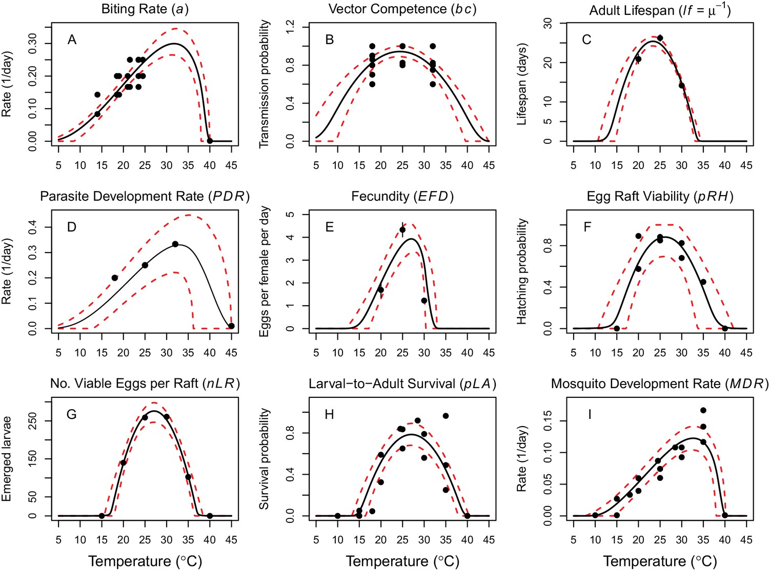
Thermal responses of Cx. annulirostris and RRV (in Ae. vigilax) traits that drive transmission.
Mosquito life history traits (A, C, E, F, G, H, I) are from Cx. annulirostris. Virus-mosquito infection traits (B, D) are from Ae. vigilax. Functions were fit using Bayesian inference with priors fit using data from other mosquito species and viruses. Black solid lines are posterior distribution means; dashed red lines are 95% credible intervals. (E, C) Points are data means; error bars are standard error. Data sources and function parameter estimates given in Figure 2—source data 1. Data sources and function parameter estimates for priors given in Figure 2—source data 2. Thermal responses fit with uniform priors given in Figure 2—figure supplement 1. Thermal responses for alternative vectors and virus given in Figure 2—figure supplements 2, 3 and 4.
-
Figure 2—source data 1
Trait thermal response functions and data sources for Ross River virus R0 models (Equations 1 and 2).
‘Par.’=model parameter. Results are given for fits from data-informed priors. Asymmetrical responses fit with Brière function (B): B(T)= qT(T – Tmin)(Tmax – T)1/2; symmetrical responses fit with quadratic function (Q): Q(T) = -q(T – Tmin)(T – Tmax). Function coefficients (and 95% credible intervals) fit via Bayesian inference.
- https://doi.org/10.7554/eLife.37762.011
-
Figure 2—source data 2
Trait thermal response functions and data sources used to parameterize priors for data-informed trait thermal responses.
‘Par.’=model parameter. Fits were made with uniform priors. Asymmetrical responses fit with Brière function (B): B(T)= qT(T – Tmin)(Tmax – T)1/2; symmetrical responses fit with quadratic function (Q): Q(T) = -q(T – Tmin)(T – Tmax). Function coefficients (and 95% credible intervals) fit via Bayesian inference.
- https://doi.org/10.7554/eLife.37762.012
Vector and pathogen traits that drive transmission consistently responded to temperature (Figure 2), though data were sparse (McDonald et al., 1980; Mottram et al., 1986; Russell, 1986; Rae, 1990; Kay and Jennings, 2002). Although we exhaustively searched for experiments with trait measurements at three or more constant temperatures in the Australian vector species (Cx. annulirostris, Ae. vigilax, Ae. camptorhynchus, Ae. notoscriptus, and Ae. normanensis), no species had data for all necessary traits (Figure 1). Thus, we combined traits from two species to build composite R0 models. We used mosquito life history traits measured in Cx. annulirostris: fecundity (as eggs per female per day, EFD), egg survival (as the proportion of rafts that hatch, pRH, and the number of larvae emerging per viable raft, nLR), the proportion surviving from larvae-to-adulthood (pLA), mosquito development rate (MDR), adult mosquito lifespan (lf), and biting rate (a). We used infection traits measured in Ae. vigilax: vector competence (bc) and parasite development rate (PDR). For comparison, we also fit traits for other mosquito and virus species: MDR and pLA from Ae. camptorhynchus and Ae. notoscriptus, and PDR and bc from Murray Valley encephalitis virus (another important pathogen transmitted by these mosquitoes in Australia) in Cx. annulirostris (Figure 2—figure supplements 2, 3 and 4) (Kay et al., 1989; Barton and Aberton, 2005; Williams and Rau, 2011). We used sensitivity analyses to evaluate the potential impact of this vector mismatch. However, all spatial and temporal predictions of R0 (Figures 5–7) use the full R0 model parameterized with mosquito life history traits from Cx. annulirostris and infection traits from Ae. vigilax (as shown in Figure 2).
Thermal optima ranged from 23.4°C for adult lifespan (lf) to 33.0°C for parasite development rate (PDR; Figure 2). The data supported unimodal thermal responses for most traits, though declines at high temperatures were not directly observed for biting rate (a) and parasite development rate. Data from other mosquito species and ectotherm physiology theory imply these traits must decline at very high temperatures, so we used strong priors to make them decline near ~40°C. Because our approach is designed to identify which traits constrain transmission at thermal limits, this choice is conservative since it means R0 will be limited by other traits with better data. Accordingly, in the absence of data we preferred to overestimate upper thermal limits and underestimate lower thermal limits rather than vice versa.
Figure 3 with 3 supplements see all
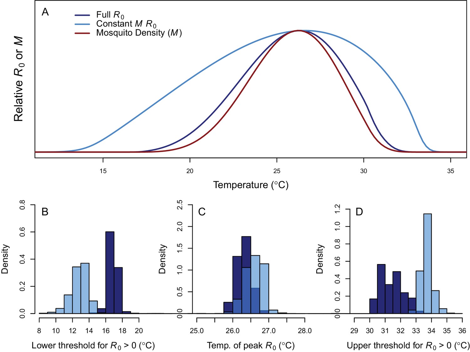
Thermal response of relative R0.
(A) Posterior means across temperature for the full R0 model (Equation 1, dark blue) and constant M model (Equation 2, light blue). Predicted mosquito density (M) shown for comparison (red). The y-axis shows relative R0 (or M) rather than absolute values, which would require additional information. Histograms of posterior distributions for (B) critical thermal minimum, (C) thermal optimum, and (D) critical thermal maximum temperatures for both models (same colors as in A). Additional R0 model results given in Figure 3—figure supplement 1. Sensitivity and uncertainty analyses given in Figure 3—figure supplement 2. Example comparison of mean and median results given in Figure 3—figure supplement 3.
Transmission potential (relative R0 from the full R0 model) peaked at 26.4°C, and was positive from 17.0–31.5°C (Figure 3). Removing the temperature-dependence of mosquito density [M] did not substantially affect the peak, because the optima for transmission and mosquito density were closely aligned (constant M model: 26.6°C, M: 26.2°C). By contrast, the range of temperatures suitable for transmission is much larger when mosquito density does not depend on temperature because M(T) constrains transmission at the thermal limits (constant M model positive from 12.9–33.7°C). The thermal constraints that mosquito density imposes on transmission are important because, although demographic traits are well-known to vary with temperature in the laboratory, many temperature-dependent transmission models do not assume that temperature influences mosquito density (Martens et al., 1997; Craig et al., 1999; Paull et al., 2017; Caminade et al., 2017; Hamlet et al., 2018, but see Parham and Michael, 2009; Mordecai et al., 2013, Mordecai et al., 2017; Johnson et al., 2015). The moderate optimal temperature for RRV (26–27°C) fits within the range of thermal optima found for other diseases: malaria transmission by Anopheles spp. at 25°C, and dengue and other viruses by Ae. aegypti and Ae. albopictus at 29 and 26°C, respectively (Figure 4) (Mordecai et al., 2013; Mordecai et al., 2017).
Figure 4
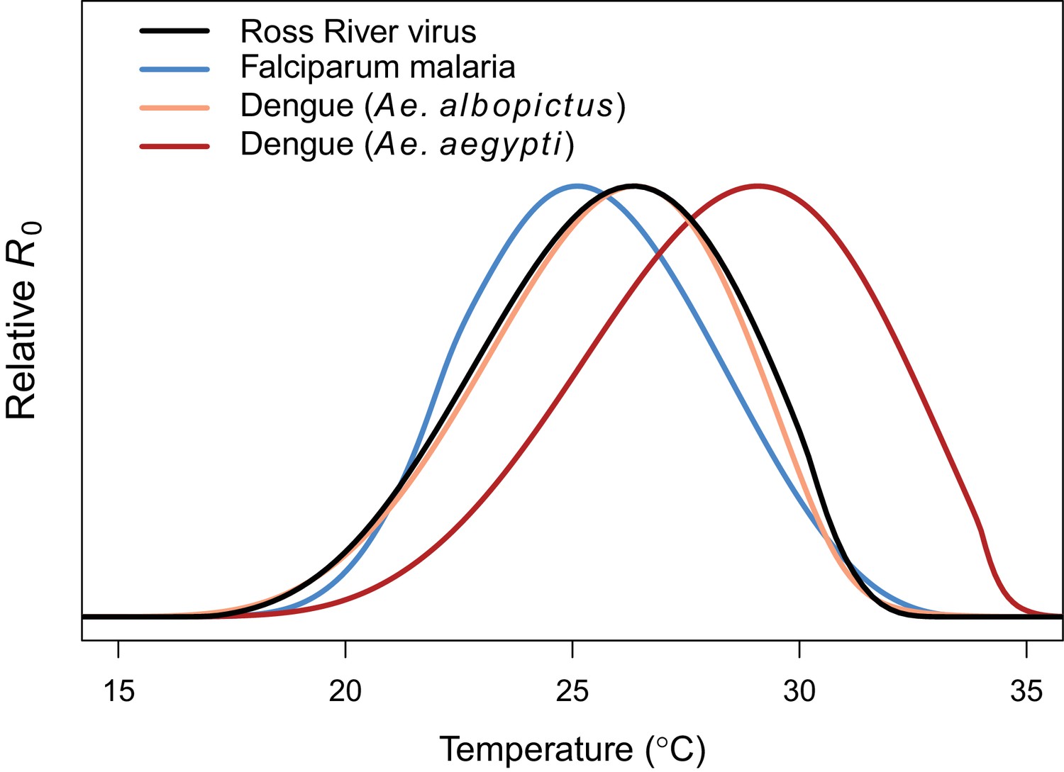
Comparing relative R0 for RRV and other diseases.
Malaria (blue, optimum = 25.2°C), Ross River virus (black, optimum = 26.4°C), dengue virus in Ae. albopictus (orange, optimum = 26.4°C), and dengue virus in Ae. agypti (red, optimum = 29.1°C). Results for all diseases use the full R0 model.
At the upper thermal limit fecundity (EFD) and adult lifespan (lf) constrain R0, while at the lower thermal limit fecundity, larval survival (pLA), egg survival (raft viability [pRH] and survival within rafts [nLR]), and adult lifespan constrain R0 (Figure 3—figure supplement 2). All of these traits (except adult lifespan) only occur in, and adult lifespan is quantitatively more important in, the full R0 model, illustrating the importance of incorporating effects of temperature on vector life history. Correspondingly, uncertainty in these traits generated the most uncertainty in R0 at the respective thermal limits (Figure 3—figure supplement 2C). The optimal temperature for R0 was most sensitive to the thermal response of adult lifespan. Near the optimum, most uncertainty in R0 was due to uncertainty in the thermal responses of biting rate and egg raft viability. For comparison, substituting larval traits from alternative vectors or infection traits for Murray Valley Encephalitis virus did not substantially alter the R0 thermal response, since Cx. annulirostris life history traits strongly constrained transmission (Figure 3—figure supplement 1).
Temperature suitability for RRV transmission varies seasonally across Australia, based on the full R0 model (Equation 1) using monthly mean temperatures from WorldClim. In subtropical and temperate locations (Brisbane and further south), low temperatures force R0 to zero for part of the year (Figures 5A and 6). Monthly mean temperatures in these areas fall along the increasing portion of the R0 curve for the entire year, so thermal suitability for transmission increases with temperature. By contrast, in tropical, northern Australia (Darwin and Cairns), the temperature remains suitable throughout the year (Figures 5 and 6). Darwin is the only major city where mean temperatures exceed the thermal optimum, and thereby depress transmission. Because most Australians live in southern, temperate areas, country-scale transmission is strongly seasonal. Using the average (1992–2013) seasonal incidence at the national scale, human cases peak two months after population-weighted R0(T), matching our a priori hypothesized time lag between temperature suitability and human cases (based on empirical work in other mosquito-borne disease systems, see Materials and methods and Discussion; Figure 7).
Figure 5 with 1 supplement see all

RRV transmission potential from monthly mean temperatures.
Color indicates number of months where (A) relative R0 >0 and (B) relative R0 >0.5. Predictions are based on the posterior median of the full R0 model (Equation 1) parameterized with trait thermal responses shown in Figure 2. Points indicate selected cities (Figure 5), scaled by the percentage of total Australian population residing in each city. Maps with 2.5% and 97.5% credible intervals are given in Figure 5—figure supplement 1.
Figure 6
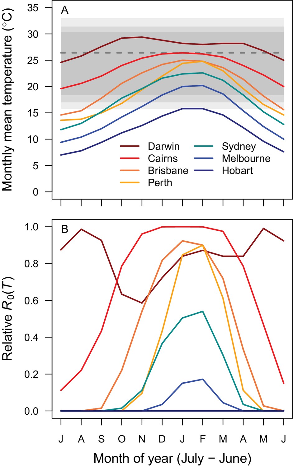
Average seasonality of temperature and relative R0 in Australian cities.
The selected cities span a latitudinal and temperature gradient (Darwin = dark red, Cairns = red, Brisbane = dark orange, Perth = light orange, Sydney = aqua, Melbourne = blue, Hobart = dark blue). The x-axis begins in July and ends in June (during winter). (A) Mean monthly temperatures. Shaded areas show temperature thresholds where R0 >0 for: outer 95% CI (light grey), median (medium grey), and inner 95% CI (dark grey). Dashed line shows median R0 optimal temperature. (B) Temperature-dependent R0. Predictions are based on the posterior median of the full R0 model (Equation 1) parameterized with trait thermal responses shown in Figure 2.
Figure 7
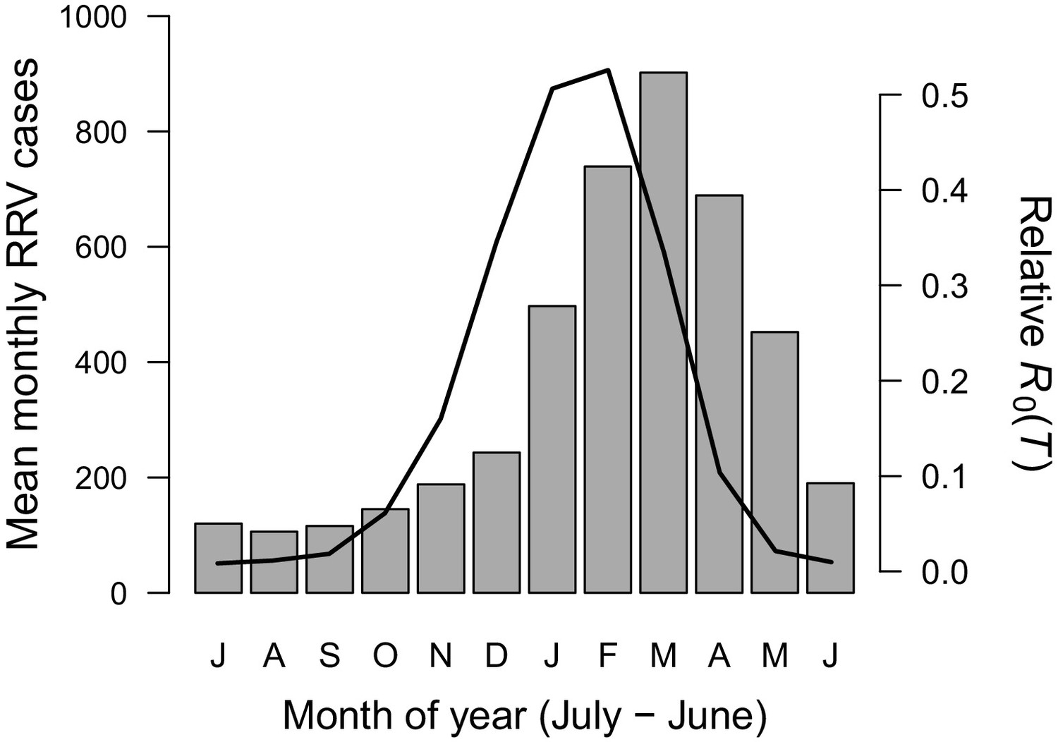
Seasonality of relative R0 and RRV infections.
Human cases aggregated nationwide from 1992 to 2013 (bars). Temperature-dependent R0 weighted by population (line), calculated from Australia’s 15 largest cities (76.6% of total population). Predictions are based on the posterior median of the full R0 model (Equation 1) parameterized with trait thermal responses shown in Figure 2. The x-axis begins in July and ends in June (during winter). Cases peak two months after R0, the a priori expected lag between temperature and reported cases.
Discussion
As the climate warms, it is critical to understand effects of temperature on transmission of mosquito-borne disease, particularly as new mosquito-borne pathogens emerge and spread worldwide. Identifying transmission optima and limits by characterizing nonlinear thermal responses, rather than simply assuming that transmission increases with temperature, can more accurately predict geographic, seasonal, and interannual variation in disease. Thermal responses vary substantially among diseases and vector species (Mordecai et al., 2013; Mordecai et al., 2017; Tesla et al., in press), yet we lack mechanistic models based on empirical, unimodal thermal responses for many diseases and vectors. Here, we parameterized a temperature-dependent model for transmission of RRV (Figure 2) with data from two important vector species (Cx. annulirostris and Ae. vigilax; Figure 1). The optimal temperature for transmission is moderate (26–27°C; Figure 3), and largely determined by the thermal response of adult mosquito lifespan (Figure 3—figure supplement 2). Both low and high temperatures limit transmission due to low mosquito fecundity and survival at all life stages—thermal responses that are often ignored in transmission models (Figure 3—figure supplement 2). Temperature explains the geography of year-round endemic versus seasonally epidemic disease (Figures 5 and 6) and accurately predicts the seasonality of human cases at the national scale (Figure 7). Thus, the model for RRV transmission provides a mechanistic link between geographic and seasonal variation in temperature and broad-scale patterns of disease.
While the thermal response of RRV transmission generally matched those of other mosquito-borne pathogens, there were some key differences. The moderate optimal temperature for RRV (26–27°C) fit within the range of thermal optima found for other diseases using the same methods: malaria transmission by Anopheles spp. at 25°C, and dengue and other viruses by Ae. aegypti and Ae. albopictus at 29 and 26°C, respectively (Figure 4) (Mordecai et al., 2013; Mordecai et al., 2017). For all of these diseases, the specific optimal temperature was largely determined by the thermal response of adult lifespan (Mordecai et al., 2013,;Mordecai et al., 2017; Johnson et al., 2015). However, the traits that set the thermal limits for RRV transmission differed from other systems. The lower thermal limit for RRV was constrained by fecundity and survival at all stages, while the upper thermal limit was constrained by fecundity and adult lifespan. By contrast, thermal limits for malaria transmission were set by parasite development rate at cool temperatures and egg-to-adulthood survival at high temperatures (Mordecai et al., 2013). As with previous models, the upper and lower thermal limits of RRV transmission are more uncertain than the optimum (Figure 3) (Johnson et al., 2015; Mordecai et al., 2017), because trait responses are harder to measure near their thermal limits where survival is low and development is slow or incomplete. Overall, our results support a general pattern of intermediate thermal optima for transmission where the well-resolved optimal temperature is driven by adult mosquito lifespan, but upper and lower thermal limits are more uncertain and may be determined by unique traits for different vector–pathogen systems. Additionally, upper thermal limits of mosquito-borne disease transmission (a major concern for climate change) are primarily determined by vector life history traits with symmetrical thermal performance curves (like fecundity and survival at various life stages) rather than rate-based traits with asymmetrical thermal performance curves (like biting rate or pathogen development rate).
The trait thermal response data were limited in two keys ways. First, two traits (fecundity and adult lifespan) had data from only three temperatures. We used priors derived from data from other mosquito species to minimize over-fitting and better represent the true uncertainty (Figure 2, versus uniform priors in Figure 2—figure supplement 1). However, data from more temperatures would increase our confidence in the fitted thermal responses. Second, no vector species had data for all traits (Figure 1), so we combined mosquito traits from Cx. annulirostris and pathogen infection traits in Ae. vigilax to build composite relative R0 models. Geographic and seasonal variation in vector populations suggests that Ae. camptorhynchus and Ae. vigilax have different thermal niches (cooler and warmer, respectively) and Cx. annulirostris has a broader thermal niche (Figure 1) (Russell, 1998). We need temperature-dependent trait data for more species to test the hypothesis that these niche differences reflect the species’ thermal responses. If true, the current model, parameterized primarily with Cx. annulirostris trait responses, may not accurately predict the thermal responses of transmission by Ae. camptorhynchus and Ae. vigilax. Hypothesized species differences in thermal niche could explain why RRV persists over a wide climatic and latitudinal gradient. Thus, thermal response experiments with other RRV vectors are a critical area for future research.
The temperature-dependent R0 model provides a mechanistic explanation for independently-observed patterns of RRV transmission across Australia. As predicted by the model (Figures 5 and 6), RRV is endemic in tropical Australia, with little seasonal variation in transmission potential due to temperature, and seasonally epidemic in subtropical and temperate Australia (Weinstein, 1997). The model also accurately predicts disease seasonality at the national scale (Figure 7), reproducing the a priori predicted lag (8–10 weeks, or 2 months) for temperature to affect reported human cases (Hu et al., 2006; Jacups et al., 2008b; Stewart Ibarra et al., 2013; Mordecai et al., 2017). This lag between temperature and reported human cases arises from the time it takes for mosquito populations to increase, bite humans and reservoir hosts, acquire RRV, become infectious, and bite subsequent hosts; for pathogens to incubate with vectors; for humans to potentially develop symptoms, seek treatment, and report cases. Further, RRV transmission by Cx. annulirostris in inland areas often moves south as temperatures increase from spring into summer (Russell, 1998), matching the model prediction (Figure 6). Although temperature is often invoked as a potential driver for these types of patterns, it is difficult to establish causality from statistical inference alone, particularly if temperature and disease both exhibit strong seasonality and could both be responding to another latent driver. Thus, the mechanistic model is a critical piece of evidence linking temperature to patterns of disease.
In addition to explaining broad-scale patterns, the unimodal thermal model explains previously contradictory local-scale results. Specifically, statistical evidence for temperature impacts on local time series of cases is mixed. RRV incidence is often—but not always—positively associated with warmer temperatures (Tong and Hu, 2001; Tong et al., 2002a; Tong et al., 2004; Hu et al., 2004; Hu et al., 2010; Jacups et al., 2008b, Williams et al., 2009; Werner et al., 2012; Koolhof et al., 2017). However, variation in the effects of temperature on transmission across space and time is expected from an intermediate thermal optimum, especially when observed temperatures are near or varying around the optimum. The strongest statistical signal of temperature on disease is expected in temperate regions where mean temperature varies along the rapidly rising portion of the R0 curve (~20–25°C). If mean temperatures vary both above and below the optimum (as in Darwin), important effects of temperature may be masked in time series models that fit linear responses. Additionally, if temperatures are always relatively suitable (as in tropical climates) or unsuitable (as in very cool temperate climates), variation in disease may be due primarily to other factors. A nonlinear mechanistic model is critical for estimating temperature impacts on transmission because the effect of increasing temperature by a few degrees can have a positive, negligible, or negative impact on R0 along different parts of the thermal response curve. Although field-based evidence for unimodal thermal responses in vector-borne disease is rare (but see Mordecai et al., 2013; Perkins et al., 2015; Peña-García et al., 2017), there is some evidence for high temperatures constraining RRV transmission and vector populations: outbreaks were less likely with more days above 35°C in part of Queensland (Gatton et al., 2005) and populations of Cx. annulirostris peaked at 25°C and declined above 32°C in Victoria (Dhileepan, 1996). Future statistical analyses of RRV cases may benefit from using a nonlinear function for temperature-dependent R0 as a predictor instead of raw temperature (Figure 6B versus Figure 6A).
Breeding habitat availability also drives mosquito abundance and mosquito-borne disease. Local rainfall or river flow have been linked to the abundance of RRV vector species (Barton et al., 2004; Tall et al., 2014; Jacups et al., 2015) and RRV disease cases (Tong and Hu, 2001; Tong et al., 2002a; Hu et al., 2004; Kelly-Hope et al., 2004b; Tong et al., 2004; Gatton et al., 2005; Jacups et al., 2008b; Bi et al., 2009; Williams et al., 2009; Werner et al., 2012), as have high tides in coastal areas with saltmarsh mosquitoes, Ae. vigilax and Ae. camptorhynchus (Tong and Hu, 2002b; Tong et al., 2004; Jacups et al., 2008b; Kokkinn et al., 2009). Overlaying models of species-specific breeding habitat with temperature-dependent models will better resolve the geographic and seasonal distribution of RRV transmission. Relative R0 peaked at similar temperatures whether or not we assumed mosquito abundance was temperature-dependent (Equation 1 versus Equation 2); however, the range of suitable temperatures was much wider for the model that assumed a temperature-independent mosquito population (Figure 3). Since breeding habitat can only impact vector populations when temperatures do not exclude them, it is critical to consider thermal constraints on mosquito abundance, even when breeding habitat is considered a stronger driver. Nonetheless, many mechanistic, temperature-dependent models of vector-borne disease transmission do not include thermal effects on vector density (Martens et al., 1997; Craig et al., 1999; Paull et al., 2017; Caminade et al., 2017; Hamlet et al., 2018). Our results demonstrate that the decision to exclude these relationships can have a critical impact on model results, especially near thermal limits.
Several important gaps remain in our understanding of RRV thermal ecology, in addition to the need for trait thermal response data for more vector species. First, the relative R0 model needs to be more rigorously validated using time series of cases to determine the importance of temperature at finer spatiotemporal scales. These analyses should incorporate daily, seasonal, and spatial temperature variation, including aquatic larval habitat and adult microhabitat temperatures (Paaijmans et al., 2010; Cator et al., 2013; Carrington et al., 2013; Thomas et al., 2018). They should also integrate species-specific drivers of breeding habitat availability, like rainfall and tidal patterns, infrastructure (e.g. drainage), and human activities (e.g. deliberate and accidental water storage). Second, translating environmental suitability for transmission into human cases also depends on disease dynamics in reservoir host populations and their impact on immunity. For instance, in Western Australia heavy summer rains can fail to initiate epidemics when low rainfall in the preceding winter depresses recruitment of susceptible juvenile kangaroos (Mackenzie et al., 2000). By contrast, large outbreaks occur in southeastern Australia when high rainfall follows a dry year, presumably from higher transmission within relatively unexposed reservoir populations (Woodruff et al., 2002). Third, as the climate changes, long-term predictions should consider potential thermal adaption of vectors, since transmission at upper thermal limits is currently limited by vector life history traits. To date, we know very little about standing genetic variation for thermal performance or existing local thermal adaptation in vectors for any disease system. Building vector species-specific R0 models and integrating thermal ecology with other drivers are important next steps for forecasting variation in RRV transmission. These more advanced models are necessary to translate our relative R0 results into predictions of absolute R0 (i.e. estimating the secondary cases per primary case, and where and when R0 >1 for sustained transmission).
Nonlinear thermal responses are particularly important for predicting how transmission will change under future climate regimes. Climate warming will likely increase the geographic and seasonal range of transmission potential in temperate, southern Australia where most Australians live. However, climate change will likely decrease transmission potential in tropical areas like Darwin, where moderate warming (~3°C) would push temperatures above the upper thermal limit for transmission for most of the year (Figure 5). However, the extent of climate-driven declines in transmission will depend on how much Cx. annulirostris and Ae. vigilax can adapt to extend their upper thermal limits and whether warmer-adapted vector species (e.g. Ae. aegypti and potentially Ae. polynesiensis) can invade and sustain RRV transmission cycles. Thus, we can predict the response of RRV transmission by current vector species to climate change based on these trait thermal responses. However, future disease dynamics will also depend on vector adaptation, potential vector species invasions, and climate change impacts on sea level and precipitation that drive vector habitat availability.
Materials and methods
Temperature-Dependent R0models
Request a detailed protocolThe ‘full R0 model’ (Equation 1) assumes temperature drives mosquito density and includes vector life history trait thermal responses (Parham and Michael, 2009; Mordecai et al., 2013; Mordecai et al., 2017). The ‘constant M model’ (Equation 2) assumes mosquito density (M) does not depend on temperature (Dietz, 1993). There is disagreement in the literature over whether the equation for R0 should contain the square root (Dietz, 1993; Heffernan et al., 2005; Smith et al., 2012). We use the version derived from the next-generation matrix method (Dietz, 1993) in order to be consistent with our previous work in other mosquito-borne disease systems (Mordecai et al., 2013; Mordecai et al., 2017; Johnson et al., 2015).
In both equations, (T) indicates that a parameter depends on temperature, a is mosquito biting rate, bc is vector competence (proportion of mosquitoes becoming infectious post-exposure), µ is adult mosquito mortality rate (adult lifespan, lf = 1/µ), PDR is parasite development rate (PDR = 1/EIP, the extrinsic incubation period), N is human density, and r is the recovery rate at which humans become immune (all rates are measured in days−1). The latter two terms do not depend on temperature. In the full R0 model, mosquito density (M) depends on fecundity (EFD, eggs per female per day), proportion surviving from egg-to-adulthood (pEA), and mosquito development rate (MDR), divided by the square of adult mortality rate (µ) (Parham and Michael, 2009). We calculated pEA as the product of the proportion of egg rafts that hatch (pRH), the number of larvae per raft (nLR, scaled by the maximum at any temperature to calculate proportional egg survival within-rafts), and the proportion of larvae surviving to adulthood (pLA).
We digitized previously published trait data (Figure 2—figure supplement 1; McDonald et al., 1980; Mottram et al., 1986; Russell, 1986; Rae, 1990; Kay and Jennings, 2002) using the free web-based tool Webplot Digitizer available at: https://automeris.io/WebPlotDigitizer/. We fit thermal responses of each trait using Bayesian inference with the ‘r2jags’ package (Plummer, 2003; Su and Yajima, 2009) in R (R Core Team, 2017). Traits with asymmetrical thermal responses were fit as Brière functions: qT(T–Tmin)(Tmax–T)1/2 (Briere et al., 1999). Traits with symmetrical thermal responses were fit as quadratic functions: -q(T–Tmin)(T–Tmax). In both functions of temperature (T), Tmin and Tmax are the critical thermal minimum and maximum, respectively, and q is a rate parameter. For priors we used gamma distributions with hyperparameters derived from thermal responses fit to data from other mosquito species (Figure 2—source data 2) (Davis, 1932; Jalil, 1972; McLean et al., 1974; Watts et al., 1987; Rueda et al., 1990; Focks et al., 1993; Joshi, 1996; Teng and Apperson, 2000; Tun-Lin et al., 2000; Alto and Juliano, 2001; Briegel and Timmermann, 2001; Kamimura et al., 2002; Calado and Navarro-Silva, 2002; Focks and Barrera, 2006; Wiwatanaratanabutr and Kittayapong, 2006; Lardeux et al., 2008; Delatte et al., 2009; Beserra et al., 2009; Yang et al., 2009; Westbrook et al., 2010; Muturi et al., 2011; Carrington et al., 2013; Tjaden et al., 2013; Eisen et al., 2014; Xiao et al., 2014; Ezeakacha, 2015; Morin et al., 2015). These priors allowed us to more accurately represent the fit and uncertainty.
Our data did not include declining trait values at high temperatures for biting rate (a) and parasite development rate (PDR). Nonetheless, data from other mosquito species (Mordecai et al., 2013; Mordecai et al., 2017) and principles of thermal biology (Dell et al., 2011) imply these traits must decline at high temperatures. Thus, for those traits we included an artificial data point where the trait value approached zero at a very high temperature (40°C), allowing us to fit the Brière function. We used strongly informative priors to limit the effect of these traits on the upper thermal limit of R0 (by constraining them to decline near 40°C). Because our approach is designed to identify which traits constrain transmission at thermal limits, this choice is conservative by allowing R0 to be limited by other traits with better data. Accordingly, in the absence of data we favored overestimating Tmax and underestimating Tmin over the alternative. For comparison, we also fit all thermal responses with uniform priors (Figure 2—figure supplement 1); these results illustrate how the priors affected the results.
Bayesian inference produces estimated posterior distributions rather than a single estimated value. Because these distributions can be non-normal and asymmetric, we report and apply medians rather than means, since medians are less sensitive to outlying values in extended tails. However, we plot mean values in the figures because they show a smoother and more visually intuitive representation of where trait and R0 thermal responses go to zero at the upper thermal limit. The means and medians are not substantially different, except at this thermal limit (see example in Figure 3—figure supplement 3).
Sensitivity and uncertainty analyses
Request a detailed protocolWe conducted sensitivity and uncertainty analyses of the full R0 model (Equation 1) to understand how trait thermal responses shape the thermal response of R0. We examined the sensitivity of R0 two ways. First, we evaluated the impact of each trait by setting it constant while allowing all other traits to vary with temperature. Second, we calculated the partial derivative of R0 with respect to each trait across temperature (∂R0/∂X · ∂X/∂T for trait X and temperature T; Equations 3-6). To understand what data would most improve the model, we also calculated the proportion of total uncertainty in R0 due to each trait across temperature. First, we propagated posterior samples from all trait thermal response distributions through to R0(T) and calculated the width of the 95% highest posterior density interval (HPD interval; a type of credible interval) of this distribution at each temperature: the ‘full R0(T) uncertainty’. Next, we sampled each trait from its posterior distribution while setting all other trait thermal responses to their posterior medians, and calculated the posterior distribution of R0(T) and the width of its 95% HPD interval across temperature: the ‘single-trait R0(T) uncertainty’. Finally, we divided each single-trait R0(T) uncertainty by the full R0(T) uncertainty.
The partial derivatives are given below for all traits (x) that appear only once in the numerator of R0 (bc, EFD, pRH, nLR, pLA, MDR; Equation 3), biting rate (a, Equation 4), parasite development rate (PDR, Equation 5), and lifespan (lf, Equation 6).
(3)
(4)
(5)
(6)
Field observations: seasonality of temperature-dependent R0across Australia
Request a detailed protocolWe took monthly mean temperatures from WorldClim for seven cities spanning a latitudinal and temperature gradient (from tropical North to temperate South: Darwin, Cairns, Brisbane, Perth, Sydney, Melbourne, and Hobart) and calculated the posterior median R0(T) for each month at each location. We also compared the seasonality of a population-weighted R0(T) and nationally aggregated RRV cases. We used 2016 estimates for the fifteen most populous urban areas, which together contain 76.6% of Australia’s population (Australian Bureau of Statistics, 2017). We calculated R0(T) for each location (as above) and estimated a population-weighted average. We compared this country-scale estimate of R0(T) with data on mean monthly human cases of RRV nationwide from 1992 to 2013 obtained from the National Notifiable Diseases Surveillance System.
We expected a time lag between temperature and reported human cases as mosquito populations increase, bite humans and reservoir hosts, acquire RRV, become infectious, and bite subsequent hosts; after an incubation period, hosts (potentially) become symptomatic, seek treatment, and report cases. Empirical work on dengue vectors in Ecuador identified a six-week time lag between temperature and mosquito oviposition (Stewart Ibarra et al., 2013). Subsequent mosquito development and incubation periods in mosquitoes and humans likely add another 2–4 week lag before cases appear, resulting in an 8–10 week lag between temperature and observed cases (Hu et al., 2006; Jacups et al., 2008b; Mordecai et al., 2017). With monthly case data, we hypothesize a two-month time lag between R0(T) and RRV disease cases.
Mapping temperature-dependent R0 across Australia
Request a detailed protocolTo illustrate temperature suitability for RRV transmission across Australia, we mapped the number of months for which relative R0(T) >0 and >0.5 for the posterior median, 2.5 and 97.5% credibility bounds (Figure 5—figure supplement 1) for the full R0 model (Equation 1). We calculated R0(T) at 0.2°C increments and projected it onto the landscape for monthly mean temperatures from WorldClim data at a 5 min resolution (approximately 10 km2 at the equator). Climate data layers were extracted for the geographic area, defined using the Global Administrative Boundaries Databases (GADM, 2012). We performed map calculations and manipulations in R with packages ‘raster’ (Hijmans, 2016), ‘maptools’ (Bivand and Lewin-Koh, 2017), and ‘Rgdal’ (Bivand et al., 2017), and rendered GeoTiffs in ArcGIS version 10.3.1.
Mosquito nomenclature
Request a detailed protocolIn 2000 there was a proposed shift in mosquito taxonomy: several subgenera within the genus Aedes were elevated to genus status (Wilkerson et al., 2015). This change affected Aedes vigilax and Aedes camptorhynchus, which were called Ochlerotataus vigilax and Ochlerotatus camptorhynchus for a time by some researchers. More recently, there has been a consensus to return to the previous naming system, so we use Aedes here, although many of the papers we cite use Ochlerotatus instead.
Additional methods for digitizing trait data
Request a detailed protocolThe fecundity and adult survival data in McDonald et al. (1980) were published as time series of one experimental population at each temperature. The resulting data needed to be transformed to fit the corresponding trait thermal responses.
For survival, McDonald et al. reported the percent surviving approximately every other day (hereafter: ‘semi-daily’). We used these data—along with the number of female adults alive on the first day of oviposition at each temperature—to generate a semi-daily time series estimating the number surviving. To generate the dataset that we used to directly fit the thermal responses, we converted this time series into the number of female individuals who died on each day (i.e. lifespan data).
For fecundity, McDonald et al. reported semi-daily fecundity data for entire population. Because the population was synchronized, and because mosquitoes lay discrete clutches of eggs separated by several days (the gonotrophic cycle duration), there were many data points when the populations did not produce offspring. These zero-inflated fecundity data are not ideal for fitting thermal responses. Therefore, after digitizing the semi-daily fecundity time series, we binned periods of several days (the bin size varied by temperature, since the gonotrophic cycle duration varies with temperature) and took a survival-weighted average within each bin (so days with more individual mothers contributing to offspring production counted more). To generate the dataset that we used to directly fit the thermal responses, we weighted the values within each bin by the mean number of surviving mothers in that bin. This approach allowed us to more accurately reflect daily fecundity averaged over a non-synchronized mosquito population. Note that the variation captured by these data and this approach is not variation between individual adult females, but rather variation by age for the whole population.
Data availability
All data and R code used for analyses in this study are included in the supporting files and also available via Dryad (http://dx.doi.org/10.5061/dryad.m0603gk).
-
Data from: Temperature explains broad patterns of Ross River virus transmissionAvailable at Dryad Digital Repository under a CC0 Public Domain Dedication.
References
-
Temperature effects on the dynamics of Aedes albopictus (Diptera: culicidae) populations in the laboratoryJournal of Medical Entomology 38:548–556.https://doi.org/10.1603/0022-2585-38.4.548
-
Report3218.0 - Regional Population Growth, Australia, 2016. CanberraAustralian Bureau of Statistics.
-
Larval development and autogeny in Ochlerotatus camptorhynchus (Thomson) (Diptera: Culicidae) from Southern VictoriaThe Proceedings of the Linnean Society of New South Wales 126:261–267.
-
Climate variability and ross river virus infections in Riverland, South Australia, 1992-2004Epidemiology and Infection 137:1486–1493.https://doi.org/10.1017/S0950268809002441
-
Links between dryland salinity, mosquito vectors, and ross river virus disease in southern inland Queensland—an example and potential implicationsAustralian Journal of Soil Research 46:62–66.https://doi.org/10.1071/SR07053
-
Rgdal: bindings for the “Geospatial” Data Abstraction LibraryRgdal: bindings for the “Geospatial” Data Abstraction Library, https://cran.r-project.org/package=rgdal.
-
Maptools: tools for reading and handling spatial objecctsMaptools: tools for reading and handling spatial objeccts, https://cran.r-project.org/package=maptools.
-
Aedes albopictus (Diptera: culicidae): physiological aspects of development and reproductionJournal of Medical Entomology 38:566–571.https://doi.org/10.1603/0022-2585-38.4.566
-
A novel rate model of Temperature-Dependent development for arthropodsEnvironmental Entomology 28:22–29.https://doi.org/10.1093/ee/28.1.22
-
A cluster of locally-acquired ross river virus infection in outer western SydneyNew South Wales Public Health Bulletin 11:132–134.https://doi.org/10.1071/NB00059
-
Some aspects of the natural history of ross river virus in South East Gippsland, victoriaArbovirus Research in Australia 5:24–28.
-
Fluctuations at a low mean temperature accelerate dengue virus transmission by Aedes aegyptiPLoS Neglected Tropical Diseases 7:e2190.https://doi.org/10.1371/journal.pntd.0002190
-
Dryland salinity and the ecology of ross river virus: the ecological underpinnings of the potential for transmissionVector-Borne and Zoonotic Diseases 9:611–622.https://doi.org/10.1089/vbz.2008.0124
-
The analysis of mortality and survival rates in wild populations of mosquitoesThe Journal of Applied Ecology 18:373–399.https://doi.org/10.2307/2402401
-
The effect of various temperatures in modifying the extrinsic incubation period of the yellow fever virus in AËDES AEGYPTI*American Journal of Epidemiology 16:163–176.https://doi.org/10.1093/oxfordjournals.aje.a117853
-
Mosquito seasonality and arboviral disease incidence in Murray Valley, southeast AustraliaMedical and Veterinary Entomology 10:375–384.https://doi.org/10.1111/j.1365-2915.1996.tb00760.x
-
The estimation of the basic reproduction number for infectious diseasesStatistical Methods in Medical Research 2:23–41.https://doi.org/10.1177/096228029300200103
-
ThesisEnvironmental Impacts and Carry-Over Effects in Complex Life Cycles: The Role of Different Life History StagesUniversity of Southern Mississippi.
-
Dynamic life table model for aedes aegypti (Diptera: culicidae): analysis of the literature and model developmentJournal of Medical Entomology 30:1003–1017.https://doi.org/10.1093/jmedent/30.6.1003
-
Report of the Scientific Working Group Meeting on Dengue92–109, Dengue transmission dynamics: assessment and implications for control, Report of the Scientific Working Group Meeting on Dengue, Geneva, WHO.
-
GADM database of Global Administrative BoundariesGADM database of Global Administrative Boundaries, 2.0, http://www.gadm.org.
-
Environmental predictors of ross river virus disease outbreaks in Queensland, AustraliaThe American Journal of Tropical Medicine and Hygiene 72:792–799.
-
The seasonal influence of climate and environment on yellow fever transmission across AfricaPLoS Neglected Tropical Diseases 12:e0006284.https://doi.org/10.1371/journal.pntd.0006284
-
Mosquito isolates of ross river virus from Cairns, Queensland, AustraliaThe American Journal of Tropical Medicine and Hygiene 62:561–565.https://doi.org/10.4269/ajtmh.2000.62.561
-
Ross river virus transmission, infection, and disease: a cross-disciplinary reviewClinical Microbiology Reviews 14:909–932.https://doi.org/10.1128/CMR.14.4.909-932.2001
-
Perspectives on the basic reproductive ratioJournal of The Royal Society Interface 2:281–293.https://doi.org/10.1098/rsif.2005.0042
-
Raster: geographic data analysis and modelingRaster: geographic data analysis and modeling, https://cran.r-project.org/package=raster.
-
Development of a predictive model for ross river virus disease in Brisbane, AustraliaThe American Journal of Tropical Medicine and Hygiene 71:.
-
Mosquito species (Diptera: culicidae) and the transmission of ross river virus in Brisbane, AustraliaJournal of Medical Entomology 43:375–381.https://doi.org/10.1093/jmedent/43.2.375
-
Bayesian spatiotemporal analysis of socio-ecologic drivers of ross river virus transmission in Queensland, AustraliaThe American Journal of Tropical Medicine and Hygiene 83:722–728.https://doi.org/10.4269/ajtmh.2010.09-0551
-
Predictive indicators for ross river virus infection in the Darwin area of tropical northern Australia, using long-term mosquito trapping dataTropical Medicine & International Health 13:943–952.https://doi.org/10.1111/j.1365-3156.2008.02095.x
-
Determining meteorological drivers of salt marsh mosquito peaks in tropical northern AustraliaJournal of Vector Ecology 40:277–281.https://doi.org/10.1111/jvec.12165
-
Effect of temperature on larval growth of aedes triseriatusJournal of Economic Entomology 65:625–626.https://doi.org/10.1093/jee/65.2.625
-
Effect of temperature on the development of Aedes aegypti and Aedes albopictusMedical Entomology and Zoology 53:53–58.https://doi.org/10.7601/mez.53.53_1
-
Differences in climatic factors between ross river virus disease outbreak and nonoutbreak yearsJournal of Medical Entomology 41:1116–1122.https://doi.org/10.1603/0022-2585-41.6.1116
-
Ross river virus disease in Australia, 1886-1998, with analysis of risk factors associated with outbreaksJournal of Medical Entomology 41:133–150.https://doi.org/10.1603/0022-2585-41.2.133
-
Ross river virus disease reemergence, Fiji, 2003-2004Emerging Infectious Diseases 11:613–615.https://doi.org/10.3201/eid1104.041070
-
Modelling the ecology of the coastal mosquitoes Aedes vigilax and Aedes camptorhynchus at Port Pirie, South AustraliaMedical and Veterinary Entomology 23:85–91.https://doi.org/10.1111/j.1365-2915.2008.00787.x
-
Fine-temporal forecasting of outbreak probability and severity: ross river virus in western AustraliaEpidemiology and Infection 145:2949–2960.https://doi.org/10.1017/S095026881700190X
-
New evidence for endemic circulation of ross river virus in the Pacific islands and the potential for emergenceInternational Journal of Infectious Diseases 57:73–76.https://doi.org/10.1016/j.ijid.2017.01.041
-
A major outbreak of Ross River virus infection in the south-west of Western Australia and the Perth metropolitan areaCommunicable Diseases Intelligence 16:290–294.
-
Ross river virus isolations from mosquitoes in arid regions of western Australia: implication of vertical transmission as a means of persistence of the virusThe American Journal of Tropical Medicine and Hygiene 49:686–696.https://doi.org/10.4269/ajtmh.1993.49.686
-
The epidemiology of outbreaks of ross river virus infection in western Australia in 1991–1992Arbovirus Research in Australia 6:72–76.
-
An outbreak of Ross River virus disease in Southwestern AustraliaEmerging Infectious Diseases 2:117–120.https://doi.org/10.3201/eid0202.960206
-
Mosquito (Diptera: Culicidae) fauna in inland areas of south-west western AustraliaAustralian Journal of Entomology 46:60–64.https://doi.org/10.1111/j.1440-6055.2007.00581.x
-
The effect of climate and weather on the transmission of ross river and murray valley encephalitis virusesMicrobiology Australia 21:20–25.
-
Outbreak of ross river virus disease in the south west districts of NSW, summer 1993New South Wales Public Health Bulletin 5:98–99.https://doi.org/10.1071/NB94037
-
Vector capability of Aedes aegypti mosquitoes for California encephalitis and dengue viruses at various temperaturesCanadian Journal of Microbiology 20:255–262.https://doi.org/10.1139/m74-040
-
Further studies on the epidemiology and effects of ross river virus in TasmaniaArbovirus Research in Australia 6:68–72.
-
A concurrent outbreak of Barmah Forest and Ross River virus disease in Nhulunbuy, Northern TerritoryCommunicable Diseases Intelligence 16:110–111.
-
Detecting the impact of temperature on transmission of Zika, dengue, and chikungunya using mechanistic modelsPLoS Neglected Tropical Diseases 11:e0005568.https://doi.org/10.1371/journal.pntd.0005568
-
Meteorologically driven simulations of dengue epidemics in San Juan, PRPLoS Neglected Tropical Diseases 9:e0004002.https://doi.org/10.1371/journal.pntd.0004002
-
The effect of temperature on eggs and immature stages of culex annulirostris skuse (Diptera: culicidae)Australian Journal of Entomology 25:131–136.https://doi.org/10.1111/j.1440-6055.1986.tb01092.x
-
Effect of temperature and insecticide stress on life-history traits of Culex restuans and Aedes albopictus (Diptera: Culicidae)Journal of Medical Entomology 48:243–250.https://doi.org/10.1603/ME10017
-
Modeling the effects of weather and climate change on malaria transmissionEnvironmental Health Perspectives 118:620–626.https://doi.org/10.1289/ehp.0901256
-
Drought and immunity determine the intensity of west nile virus epidemics and climate change impactsProceedings of the Royal Society B: Biological Sciences 284:20162078.https://doi.org/10.1098/rspb.2016.2078
-
Estimating effects of temperature on dengue transmission in colombian citiesAnnals of Global Health 83:509–518.https://doi.org/10.1016/j.aogh.2017.10.011
-
ConferenceJAGS: a program for analysis of bayesian graphical models using gibbs samplingDSC 2003. pp. 1–10.
-
SoftwareR: A Language and for Statistical ComputingR Foundation for Statistical Computing, Vienna, Austria.
-
Ross River virus in mosquitoes (Diptera: Culicidae) during the 1994 epidemic around Brisbane, AustraliaJournal of Medical Entomology 34:156–159.https://doi.org/10.1093/jmedent/34.2.156
-
Climate change and vector-borne diseasesAdvances in Parasitology 62:345–381.https://doi.org/10.1016/S0065-308X(05)62010-6
-
Epidemic polyarthritis (Ross river) virus infection in the cook islandsThe American Journal of Tropical Medicine and Hygiene 30:1294–1302.https://doi.org/10.4269/ajtmh.1981.30.1294
-
Temperature-dependent development and survival rates of Culex quinquefasciatus and Aedes aegypti (Diptera: culicidae)Journal of Medical Entomology 27:892–898.https://doi.org/10.1093/jmedent/27.5.892
-
Culex annulirostris skuse (Diptera: culicidae) AT Appin, N. S. W. – bionomics and behaviourAustralian Journal of Entomology 25:103–109.https://doi.org/10.1111/j.1440-6055.1986.tb01087.x
-
Mosquito (Diptera: culicidae) and arbovirus activity on the South coast of New South Wales, Australia, in 1985-1988Journal of Medical Entomology 28:796–804.https://doi.org/10.1093/jmedent/28.6.796
-
Ross river virus: disease trends and vector ecology in AustraliaBulletin of the Society of Vector Ecologists 19:73–81.
-
Mosquito-borne arboviruses in Australia: the current scene and implications of climate change for human healthInternational Journal for Parasitology 28:955–969.https://doi.org/10.1016/S0020-7519(98)00053-8
-
Ross river virus: ecology and distributionAnnal Reviews Entomology 47:1–31.https://doi.org/10.1146/annurev.ento.47.091201.145100
-
Definition of ross river virus vectors at Maroochy Shire, AustraliaJournal of Medical Entomology 37:146–152.https://doi.org/10.1603/0022-2585-37.1.146
-
Evaluation of three traps for sampling Aedes polynesiensis and other mosquito species in american SamoaJournal of the American Mosquito Control Association 24:319–322.https://doi.org/10.2987/5652.1
-
Temperature and population density determine reservoir regions of seasonal persistence in highland malariaProceedings of the Royal Society B: Biological Sciences 282:20151383.https://doi.org/10.1098/rspb.2015.1383
-
Climate and non-climate drivers of dengue epidemics in southern coastal EcuadorThe American Journal of Tropical Medicine and Hygiene 88:971–981.https://doi.org/10.4269/ajtmh.12-0478
-
Ross river virus disease activity associated with naturally occurring nontidal flood events in Australia: a systematic reviewJournal of Medical Entomology 51:1097–1108.https://doi.org/10.1603/ME14007
-
Extrinsic incubation period of dengue: knowledge, backlog, and applications of temperature dependencePLoS Neglected Tropical Diseases 7:e2207.https://doi.org/10.1371/journal.pntd.0002207
-
Climate variation and incidence of ross river virus in Cairns, Australia: a time-series analysisEnvironmental Health Perspectives 109:1271–1273.https://doi.org/10.1289/ehp.011091271
-
Climate variability and ross river virus transmissionJournal of Epidemiology & Community Health 56:617–621.https://doi.org/10.1136/jech.56.8.617
-
Different responses of ross river virus to climate variability between coastline and inland cities in Queensland, AustraliaOccupational and Environmental Medicine 59:739–744.https://doi.org/10.1136/oem.59.11.739
-
Climate variability and ross river virus transmission in Townsville region, Australia, 1985-1996Tropical Medicine and International Health 9:298–304.https://doi.org/10.1046/j.1365-3156.2003.01175.x
-
Effect of temperature on the vector efficiency of Aedes aegypti for dengue 2 virusThe American Journal of Tropical Medicine and Hygiene 36:143–152.https://doi.org/10.4269/ajtmh.1987.36.143
-
An ecological approach to public health intervention: ross river virus in AustraliaEnvironmental Health Perspectives 105:364–366.https://doi.org/10.1289/ehp.97105364
-
Larval environmental temperature and the susceptibility of Aedes albopictus Skuse (Diptera: Culicidae) to Chikungunya virusVector-Borne and Zoonotic Diseases 10:241–247.https://doi.org/10.1089/vbz.2009.0035
-
The epidemiology of arbovirus infection in the northern territory 1980-92Arbovirus Research in Australia 6:266–270.
-
Confirmed case of ross river virus infection acquired in alice springs march 1995The Northern Territory Communicable Disease Bulletin 2:9–11.
-
Ross river virus transmission in Darwin, Northern Territory, AustraliaArbovirus Research in Australia 7:337–345.
-
Environmental and entomological factors determining ross river virus activity in the river murray valley of South AustraliaAustralian and New Zealand Journal of Public Health 33:284–288.https://doi.org/10.1111/j.1753-6405.2009.00390.x
-
Effects of temephos and temperature on Wolbachia load and life history traits of Aedes albopictusMedical and Veterinary Entomology 20:300–307.https://doi.org/10.1111/j.1365-2915.2006.00640.x
-
Assessing the effects of temperature on the population of Aedes aegypti, the vector of dengueEpidemiology and Infection 137:1188–1202.https://doi.org/10.1017/S0950268809002040
Article and author information
Author details
Marta Strecker Shocket

Funding
National Science Foundation (DEB-1518681)
- Erin A Mordecai
National Science Foundation (DEB-1640780)
- Erin A Mordecai
The funders had no role in study design, data collection and interpretation, or the decision to submit the work for publication.
Acknowledgements
We thank Leah Johnson and Matt Thomas for comments and Cameron Webb for posting the RRV case data (https://cameronwebb.wordpress.com/2014/04/09/why-is-mosquito-borne-disease-risk-greater-in-autumn/). All authors were supported by the National Science Foundation (DEB-1518681; https://nsf.gov/). EAM was supported by the NSF (DEB-1640780; https://nsf.gov/), the Stanford Woods Institute for the Environment (https://woods.stanford.edu/research/environmental-venture-projects), and the Stanford Center for Innovation in Global Health (http://globalhealth.stanford.edu/research/seed-grants.html).
Copyright
© 2018, Shocket et al.
This article is distributed under the terms of the Creative Commons Attribution License, which permits unrestricted use and redistribution provided that the original author and source are credited.
Metrics
-
- 3,486
- views
-
- 361
- downloads
-
- 90
- citations
Views, downloads and citations are aggregated across all versions of this paper published by eLife.
Citations by DOI
-
- 90
- citations for umbrella DOI https://doi.org/10.7554/eLife.37762
Download links
A two-part list of links to download the article, or parts of the article, in various formats.
Downloads (link to download the article as PDF)
Open citations (links to open the citations from this article in various online reference manager services)
Cite this article (links to download the citations from this article in formats compatible with various reference manager tools)
Temperature explains broad patterns of Ross River virus transmission
eLife 7:e37762.
https://doi.org/10.7554/eLife.37762


