Figures and data in How biological attention mechanisms improve task performance in a large-scale visual system model | eLife

Figures
Additional files

9 figures and 1 additional file

Figures

Figure 1

Download asset Open asset

Network architecture and feature-based attention task setup.

(A) The model used is a pre-trained deep neural network (VGG-16) that contains 13 convolutional layers (labelled in gray, number of feature maps given in parenthesis) and is trained on the ImageNet dataset to do 1000-way object classification. All convolutional filters are 3 × 3. (B) Modified architecture for feature-based attention tasks. To perform our feature-based attention tasks, the final layer that was implementing 1000-way softmax classification is replaced by binary classifiers (logistic regression), one for each category tested (two shown here, 20 total). These binary classifiers are trained on standard ImageNet images. (C) Test images for feature-based attention tasks. Merged images (left) contain two transparently overlaid ImageNet images of different categories. Array images (right) contain four ImageNet images on a 2 × 2 grid. Both are 224 × 224 pixels. These images are fed into the network and the binary classifiers are used to label the presence or absence of the given category. (D) Performance of binary classifiers. Box plots describe values over 20 different object categories (median marked in red, box indicates lower to upper quartile values and whiskers extend to full range, with the exception of outliers marked as dots). ‘Standard’ images are regular ImageNet images not used in the binary classifier training set.

https://doi.org/10.7554/eLife.38105.003

Figure 2

Download asset Open asset

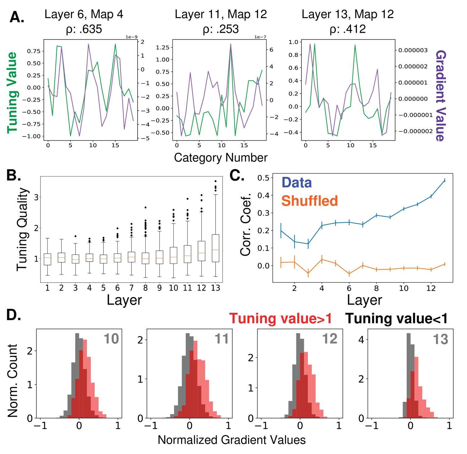
Relationship between feature map tuning and gradient values.

(A) Example tuning values (green, left axis) and gradient values (purple, right axis) of three different feature maps from three different layers (identified in titles, layers as labelled in Figure 1A) over the 20 tested object categories. Tuning values indicate how the response to a category differs from the mean response; gradient values indicate how activity should change in order to classify input as from the category. Correlation coefficients between tuning curves and gradient values given in titles. All gradient and tuning values available in Figure 2—source data 1 (B) Tuning quality across layers. Tuning quality is defined per feature map as the maximum absolute tuning value of that feature map. Box plots show distribution across feature maps for each layer. Average tuning quality for shuffled data: .372 ± .097 (this value does not vary significantly across layers) (C) Correlation coefficients between tuning curves and gradient value curves averaged over feature maps and plotted across layers (errorbars ± S.E.M., data values in blue and shuffled controls in orange). (D) Distributions of gradient values when tuning is strong. In red, histogram of gradient values associated with tuning values larger than one (i.e. for feature maps that strongly prefer the category), across all feature maps in layers 10, 11, 12, and 13. For comparison, histograms of gradient values associated with tuning values less than one are shown in black (counts are separately normalized for visibility, as the population in black is much larger than that in red).

https://doi.org/10.7554/eLife.38105.004

Figure 2—source data 1 Object tuning curves and gradients.: https://doi.org/10.7554/eLife.38105.005
Download elife-38105-fig2-data1-v2.txt

Figure 3 with 2 supplements

Download asset Open asset

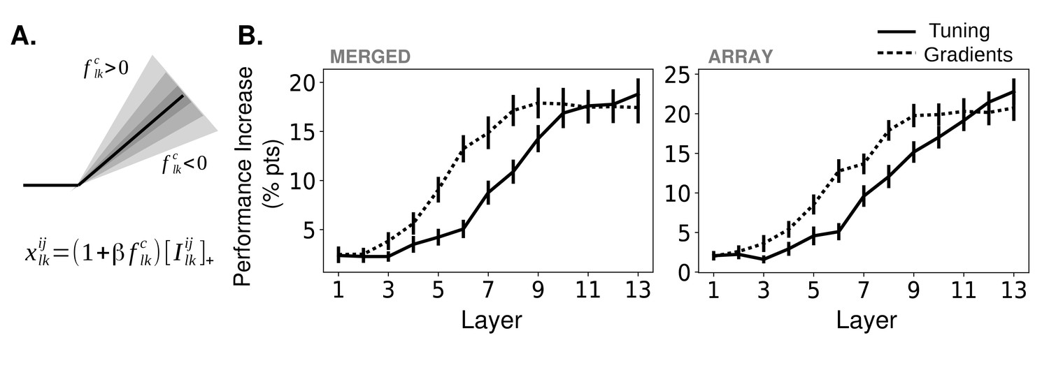
Effects of applying feature-based attention on object category tasks.

(A) Schematic of how attention modulates the activity function. All units in a feature map are modulated the same way. The slope of the activation function is altered based on the tuning (or gradient) value, $f_{l k}^{c}$ , of a given feature map (here, the $k^{t h}$ feature map in the $l^{t h}$ layer) for the attended category, $c$ , along with an overall strength parameter $β$ . $I_{l k}^{i j}$ Is the input to this unit from the previous layer. For more information, see Materials and methods, 'How attention is applied'. (B) Average increase in binary classification performance as a function of layer at which attention is applied (solid line represents using tuning values, dashed line using gradient values, errorbars ± S.E.M.). In all cases, best performing strength from the range tested is used for each instance. Performance shown separately for merged (left) and array (right) images. Gradients perform significantly ( $p < .05$ , $N = 20$ ) better than tuning at layers 5 – 8 (p=4.6e^-3, 2.6e^-5, 6.5e^-3, 4.4e^-3) for merged images and 5 – 9 (p=3.1e^-2, 2.3e^-4, 4.2e^-2, 6.1e^-3, 3.1e^-2) for array images. Raw performance values in Figure 3—source data 1.

https://doi.org/10.7554/eLife.38105.006

Figure 3—source data 1 Performance changes with attention.: https://doi.org/10.7554/eLife.38105.009
Download elife-38105-fig3-data1-v2.txt

Figure 3—figure supplement 1

Download asset Open asset

Effect of applying attention to all layers or all feature maps uniformly.

(A) Effect of applying attention at all layers simultaneously for the category detection task. Performance increase in merged (left) and array (right) image tasks when attention is applied with tuning curves (red) or gradients (blue). Range of strengths tested is one-tenth that of the range tested when applying attention at only one layer and best-performing strength for each category is used. Errorbars are ± S.E.M. (B) Same as (A) but for orientation detection task (Figure 5A) (C) Control experiment. Instead of using tuning values or gradient values to determine how activity modulates feature maps, all feature maps are scaled by the same amount. Best-performing strengths are used for each category. These results show that merely scaling activity is insufficient to create the performance gains seen when attention is applied in a specific manner. Note: these results are independent of the layer at which the modulation takes place because ${[(1 + β) * I_{l k}^{i j}]}_{+} = (1 + β) {[I_{l k}^{i j}]}_{+}$ if $(1 + β) > 0$ .

https://doi.org/10.7554/eLife.38105.007

Figure 3—figure supplement 2

Download asset Open asset

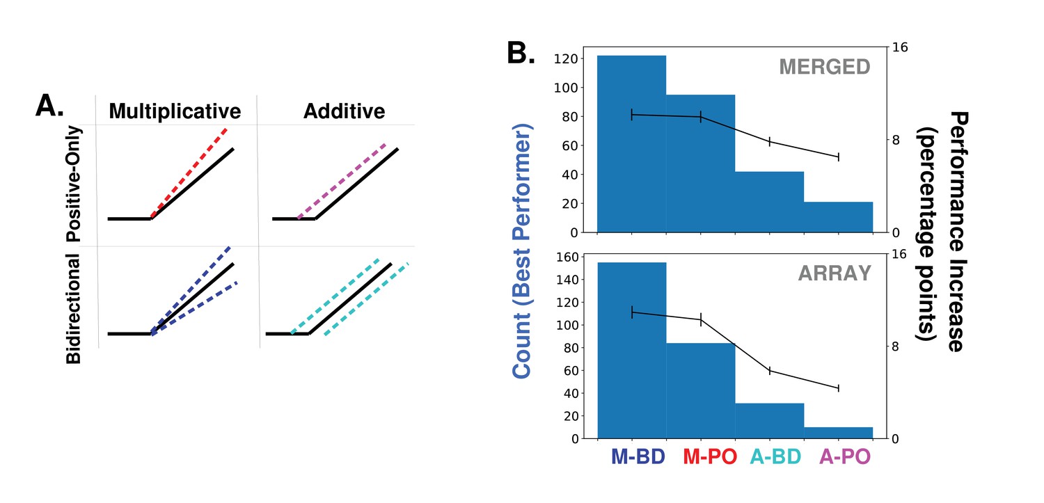
Alternative forms of attention.

(A) Schematics of how attention can modulate the activity function. Feature-based attention modulates feature maps according to their tuning values but this modulation can scale the activity multiplicatively or additively, and can either only enhance feature maps that prefer the attended category (positive-only) or also decrease the activity of feature maps that do not prefer it (bidirectional). See Materials and methods, 'Implementation options' for details of these implementations. The main body of this paper only uses multiplicative bi-directional attention. (B) Comparison of binary classification performance when attention is applied in each of the four ways described in (A). Considering the combination of attention applied to a given category at a given layer/layers as an instance (20 categories * 14 layer options = 280 instances), histograms (left axis) show how often the given option is the best performing, for merged (top) and array (bottom) images. Average increase in binary classification performance for each option also shown (right axis, averaged across all instances, errorbars ± S.E.M.).

https://doi.org/10.7554/eLife.38105.008

Figure 4 with 1 supplement

Download asset Open asset

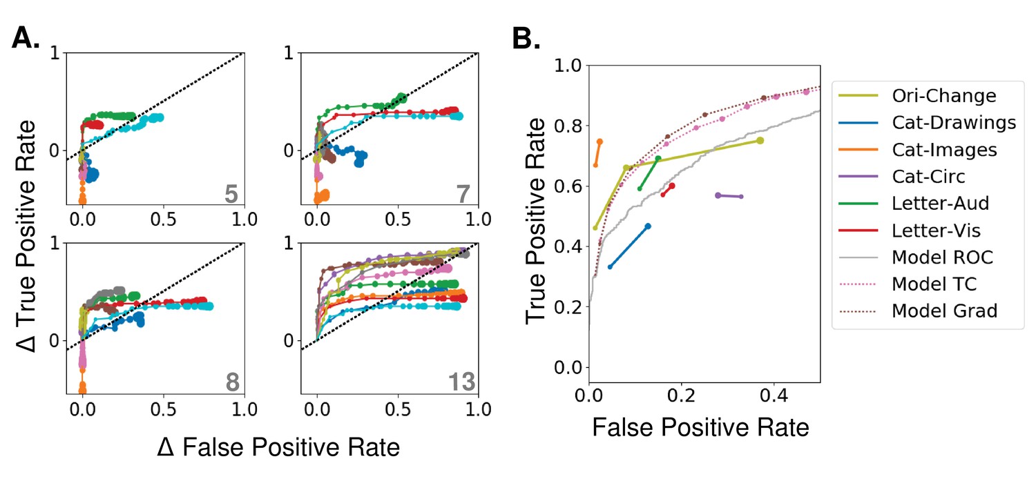
Effects of varying attention strength

(A) Effect of increasing attention strength ( $β$ ) in true and false positive rate space for attention applied at each of four layers (layer indicated in bottom right of each panel, attention applied using tuning values). Each line represents performance for an individual category (only 10 categories shown for visibility), with each increase in dot size representing a .15 increase in $β$ . Baseline (no attention) values are subtracted for each category such that all start at (0,0). The black dotted line represents equal changes in true and false positive rates. (B) Comparisons from experimental data. The true and false positive rates from six experiments in four previously published studies are shown for conditions of increasing attentional strength (solid lines). Cat-Drawings = (Lupyan and Ward, 2013), Exp. 1; Cat-Images=(Lupyan and Ward, 2013),Exp. 2; Objects=(Koivisto and Kahila, 2017), Letter-Aud.=(Lupyan and Spivey, 2010), Exp. 1; Letter-Vis.=(Lupyan and Spivey, 2010), Exp. 2. Ori-Change=(Mayo and Maunsell, 2016). See Materials and methods, 'Experimental data' for details of experiments. Dotted lines show model results for merged images, averaged over all 20 categories, when attention is applied using either tuning (TC) or gradient (Grad) values at layer 13. Model results are shown for attention applied with increasing strengths (starting at 0, with each increasing dot size representing a .15 increase in $β$ ). Receiver operating curve (ROC) for the model using merged images, which corresponds to the effect of changing the threshold in the final, readout layer, is shown in gray. Raw performance values in Figure 3—source data 1.

https://doi.org/10.7554/eLife.38105.010

Figure 4—figure supplement 1

Download asset Open asset

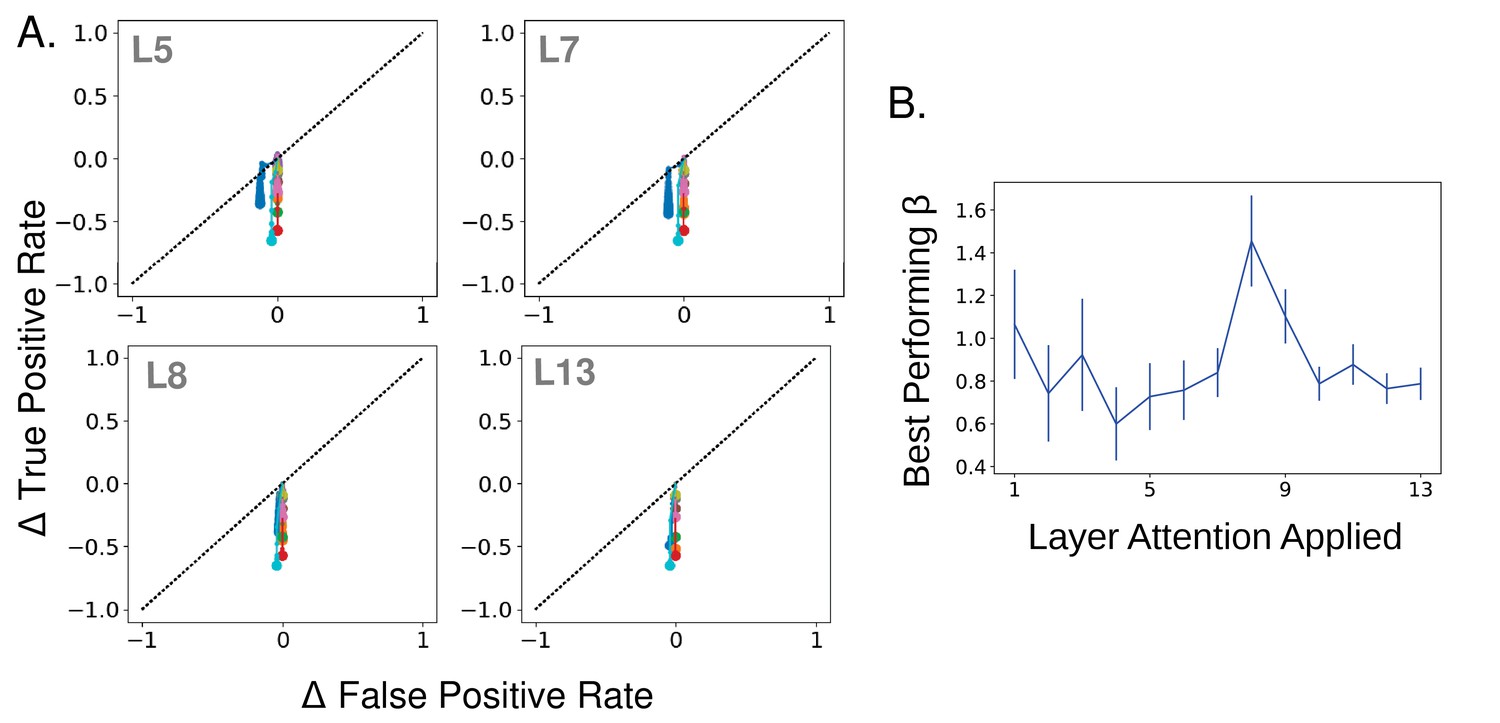
Negatively applying attention and best-performing strengths.

(A) Effect of strength increase in true and false positive rate space when tuning values are negated. Negated tuning values have the same overall level of positive and negative modulation but in the opposite direction of tuning for a given category. Plot same as in Figure 4A. Layer attention applied at indicated in gray. Attention applied in this way decreases true positives, and to a lesser extent false positives (the initial false positive rate when no attention is applied is very low). (B) Mean best performing strength ( $β$ value; using regular non-negated attention) across categories as a function of the layer attention is applied at, according to merged images task. Errorbars ± S.E.M.

https://doi.org/10.7554/eLife.38105.011

Figure 5 with 1 supplement

Download asset Open asset

Attention task and results using oriented gratings.

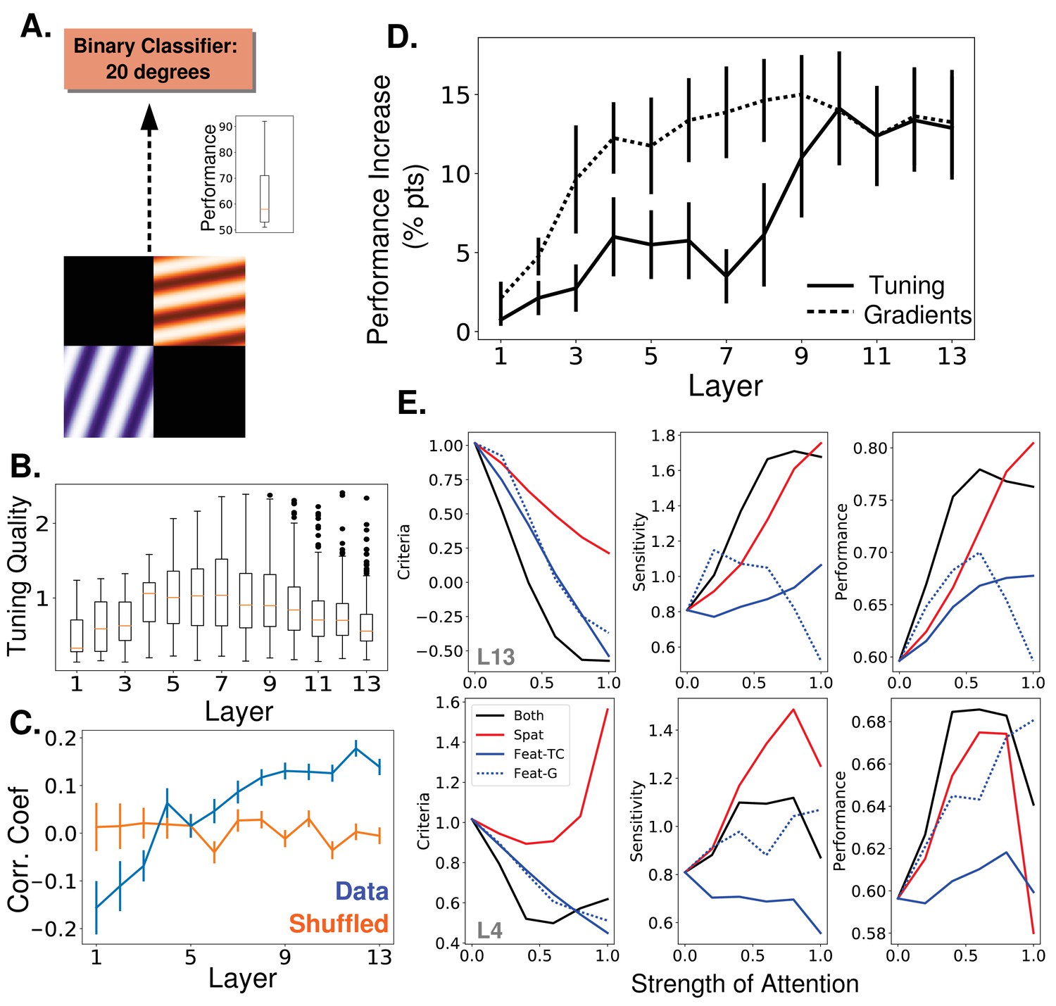
(A) Orientation detection task. Like with the object category detection tasks, separate binary classifiers trained to detect each of 9 different orientations replaced the final layer of the network. Test images included two oriented gratings of different color and orientation located at 2 of 4 quadrants. Inset shows performance over nine orientations without attention (B) Orientation tuning quality as a function of layer. (C) Average correlation coefficient between orientation tuning curves and gradient curves across layers (blue). Shuffled correlation values in orange. Errorbars are ± S.E.M. (D) Comparison of performance on orientation detection task when attention is determined by tuning values (solid line) or gradient values (dashed line) and applied at different layers. As in Figure 3B, best performing strength is used in all cases. Errorbars are ±S.E.M. Gradients perform significantly (p=1.9e -2) better than tuning at layer 7. Raw performance values available in Figure 5—source data 1. (E) Change in signal detection values and performance (perent correct) when attention is applied in different ways—spatial (red), feature according to tuning (solid blue), feature according to gradients (dashed blue), and both spatial and feature (according to tuning, black)—for the task of detecting a given orientation in a given quadrant. Top row is when attention is applied at layer 13 and bottom when applied at layer 4. Raw performance values available in Figure 5—source data 2.

https://doi.org/10.7554/eLife.38105.012

Figure 5—source data 1 Performance on orientation detection task.: https://doi.org/10.7554/eLife.38105.014
Download elife-38105-fig5-data1-v2.txt
Figure 5—source data 2 Performance on spatial and feature-based attention task.: https://doi.org/10.7554/eLife.38105.015
Download elife-38105-fig5-data2-v2.txt

Figure 5—figure supplement 1

Download asset Open asset

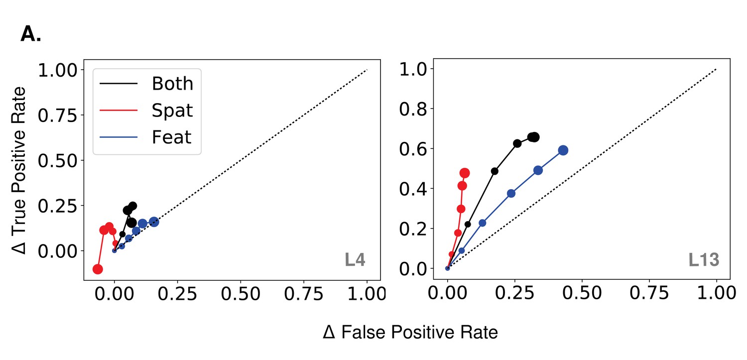
True and false positive changes with spatial and feature-based attention.

(A) Effect of strength increase in true and false positive rate space when attention is applied according to quadrant, orientation, or both in the orientation detection task. Rates averaged over orientations/locations. Increasing dot size corresponds to .2 increase in $β$ each. No-attention rates are subtracted and the black dotted line indicates equal increase in true and false positives. Layer attention applied at indicated in gray.

https://doi.org/10.7554/eLife.38105.013

Figure 6 with 2 supplements

Download asset Open asset

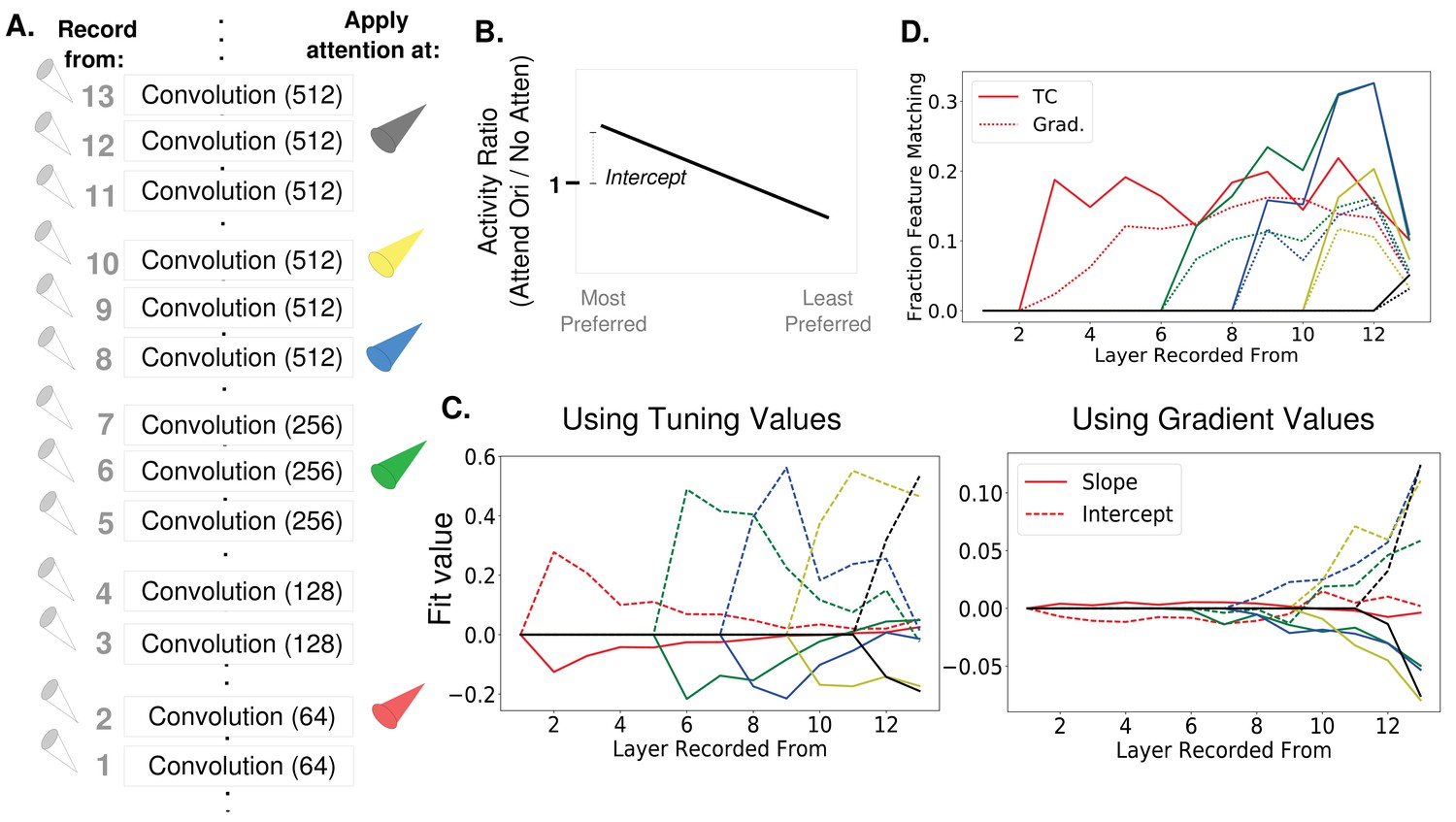
How attention-induced activity changes propagate through the network.

(A) Recording setup. The spatially averaged activity of feature maps at each layer was recorded (left) while attention was applied at layers 2, 6, 8, 10, or 12 individually. Activity was in response to a full field oriented grating. (B) Schematic of metric used to test for the feature similarity gain model. Activity when a given orientation is present and attended is divided by the activity when no attention is applied, giving a set of activity ratios. Ordering these ratios from most to least preferred orientation and fitting a line to them gives the slope and intercept values plotted in (C). Intercept values are plotted in terms of how they differ from 1, so positive values are an intercept greater than 1. (FSGM predicts negative slope and positive intercept). (C) The median slope (solid line) and intercept (dashed line) values as described in (B) plotted for each layer when attention is applied to the layer indicated by the line color as labelled in (A). On the left, attention applied according to tuning values and on the right, attention applied according to gradient values. Raw slope and intercept values when using tuning curves available in Figure 6—source data 1 and for gradients in Figure 6—source data 2. (D) Fraction of feature maps displaying feature matching behaviour at each layer when attention is applied at the layer indicated by line color. Shown for attention applied according to tuning (solid lines) and gradient values (dashed line).

https://doi.org/10.7554/eLife.38105.016

Figure 6—source data 1 Intercepts and slopes from gradient-applied attention.: https://doi.org/10.7554/eLife.38105.019
Download elife-38105-fig6-data1-v2.txt
Figure 6—source data 2 Intercepts and slopes from tuning curve-applied attention.: https://doi.org/10.7554/eLife.38105.020
Download elife-38105-fig6-data2-v2.txt

Figure 6—figure supplement 1

Download asset Open asset

Feature-based attention at one layer often suppresses activity of the attended features at later layers.

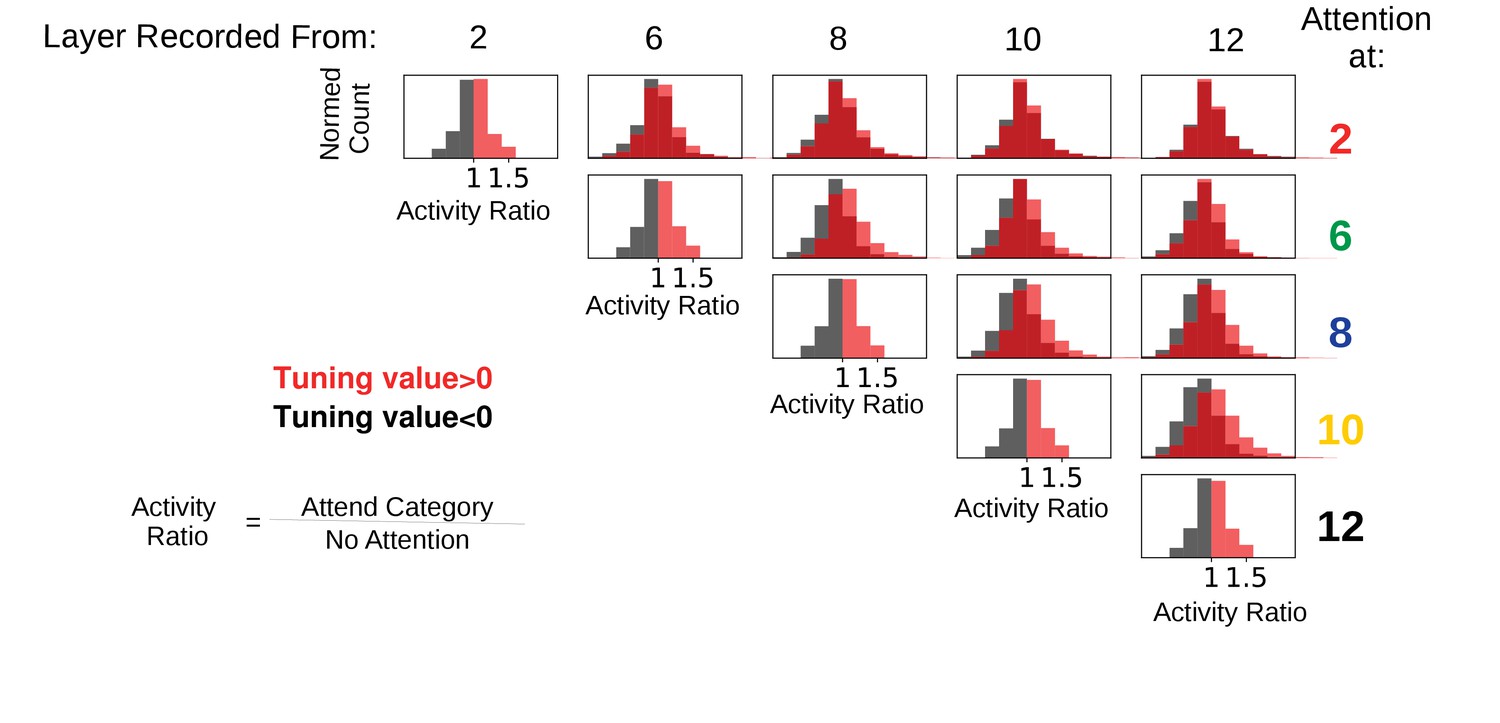
Activity ratios are shown for when attention is applied (according to tuning) at various layers individually and activity is recorded from that layer and later layers. In all cases, the category attended was the same as the one present in the input image (standard ImageNet images used to ensure that these results are not influenced by the presence of other category features in the input). Histograms are of ratios of feature map activity when attention is applied to the category divided by activity when no attention is applied, split according to whether the feature map prefers (red) or does not prefer (black) the attended category. In many cases, feature maps that prefer the attended category have activity ratios less than one, indicating that attention at a lower layer decreases the activity of feature maps that prefer the attended category. The misalignment between lower and later layers is starker the larger the distance between the attended and recorded layers. For example, when looking at layer 12, attention applied at layer two appears to increase and decrease feature map activity equally, without respect to category preference. This demonstrates the ability of attention at a lower layer to change activity in ways opposite to the effects of attention at the recorded layer.

https://doi.org/10.7554/eLife.38105.017

Figure 6—figure supplement 2

Download asset Open asset

Correlating activity changes with performance changes.

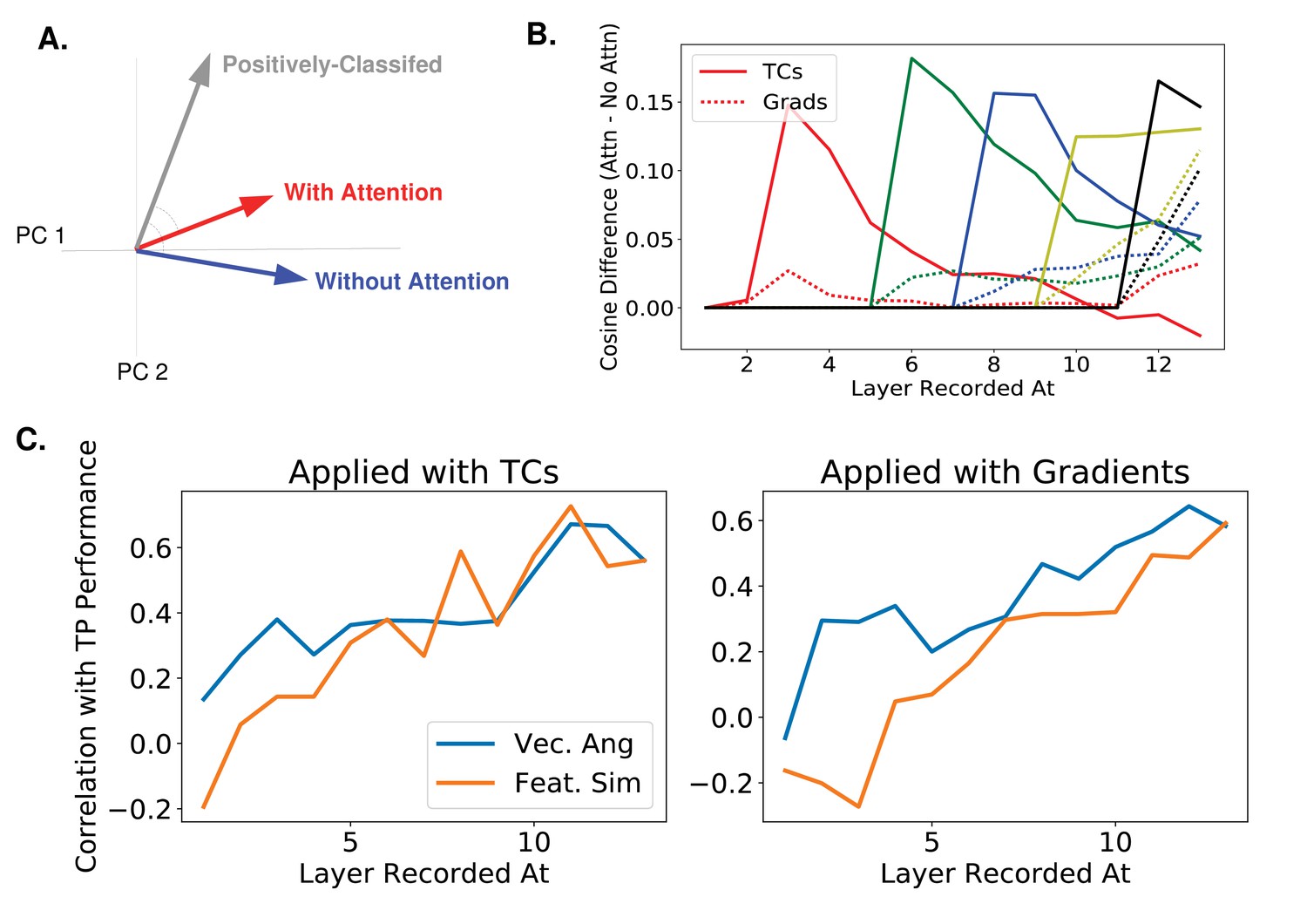
(A) A new measure of activity changes inspired by gradient values. The gray vector represents the average pattern of neural activity in response to images the classifier indicates as containing the given orientation (i.e., positively-classified in the absence of attention, whether or not the orientation was present in the image). The blue vector (activity without attention) and red vector (activity when attention is applied) are then made using images that do contain the given orientation. Assuming that attention makes activity look more like activity during positive classification, this measure compares the cosine of the angle between the positively-classified and with-attention vectors to the cosine of the angle between the positively-classified and without-attention vectors. We use $\cos θ$ as the measure, but results are similar using $θ$ . See Materials and methods, 'Correlating activity changes with performance' for how this is calculated (B) Using the same color scheme as Figure 6, this plot shows how attention applied at different layers causes activity changes throughout the network, as measured by the vector method introduced in (A). Specifically, the cosine of the angle between the positively-classified and without-attention vectors is subtracted from the cosine of the angle between the positively-classified and with-attention vectors. Solid lines indicate median value of this difference (across images) when attention is applied with tuning curves and dashed line when applied with gradients. (C) How activity changes correlate with performance changes. The correlation coefficient between the change in true positive rate with attention and activity changes as measured by: difference in cosines of angles (blue line) or feature similarity gain model-like behaviour (orange line). Activity and performance changes are collected when attention is applied at different layers individually (using a range of strengths) according to tuning curves (left) or gradient values (right). Activity is recorded at and after the layer at which attention is applied. For a given layer L, the correlation coefficient is thus computed across data points, where there is one data point for each combination of orientation, strength of attention applied, and layer (l $\leq$ L) at which attention is applied. A bootstrap analysis determined that at layers 1, 2, 3, 4, and 5 the vector angle method had significantly ( $p < .05$ ) higher correlation with performance for both application options than the FSGM measure.

https://doi.org/10.7554/eLife.38105.018

Figure 7

Download asset Open asset

A proposed experiment to distinguish between tuning-based and gradient-based attention

(A) ‘Cross-featural’ attention task. Here, the final layer of the network is replaced with a color classifier and the task is to classify the color of the attended orientation in a two-orientation stimulus. Importantly, in both this and the orientation detection task (Figure 5A), a subject performing the task would be cued to attend to an orientation. (B) The correlation coefficient between the gradient values calculated for this task and orientation tuning values (as in Figure 5C). Correlation peaks at lower layers for this task. (C) Correlation between tuning values for the two tasks (blue) and between gradient values for the two tasks (orange). If attention does target cells based on tuning, the modulation would be the same in both the color classification task and the orientation detection task. If a gradient-based targeting is used, no (or even a slight anti-) correlation is expected. Tuning and gradient values available in Figure 7—source data 1.

https://doi.org/10.7554/eLife.38105.021

Figure 7—source data 1 Orientation tuning curves and gradients.: https://doi.org/10.7554/eLife.38105.022
Download elife-38105-fig7-data1-v2.txt

Author response image 1

Download asset Open asset

https://doi.org/10.7554/eLife.38105.025

Author response image 2

Download asset Open asset

https://doi.org/10.7554/eLife.38105.026

Additional files

Transparent reporting form: https://doi.org/10.7554/eLife.38105.023
Download elife-38105-transrepform-v2.pdf

Download links

A two-part list of links to download the article, or parts of the article, in various formats.

Downloads (link to download the article as PDF)

Open citations (links to open the citations from this article in various online reference manager services)

Mendeley

Cite this article (links to download the citations from this article in formats compatible with various reference manager tools)

Grace W Lindsay
Kenneth D Miller

(2018)

How biological attention mechanisms improve task performance in a large-scale visual system model

eLife 7:e38105.

https://doi.org/10.7554/eLife.38105

Sign up for email alerts

Privacy notice