A kinematic synergy for terrestrial locomotion shared by mammals and birds
- University of Rome Tor Vergata, Italy
- IRCCS Santa Lucia Foundation, Italy
Figures
Figure 1
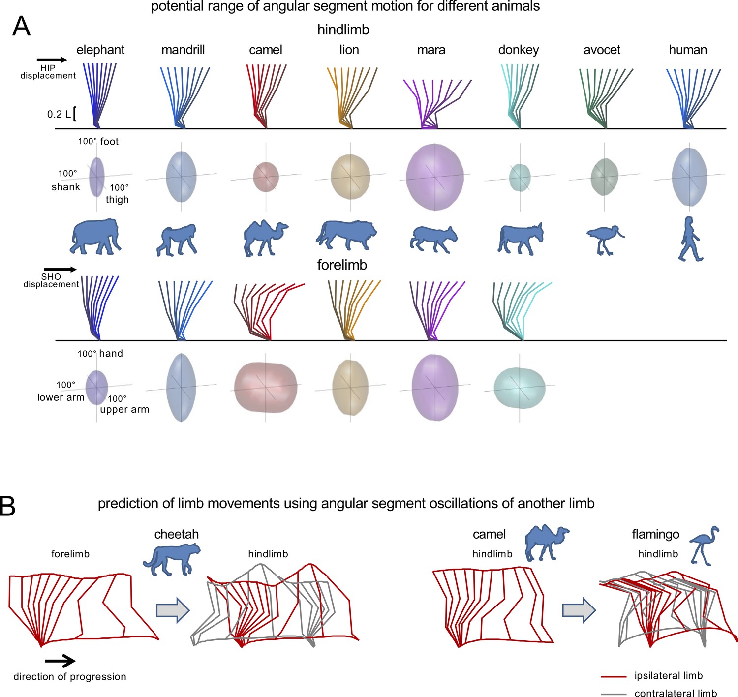
Interspecific comparison of angular movements during walking using a tri-segmented limb model.
(A) Potential range of angular segment motion for representative animals of different orders during stance assuming a fixed endpoint and constant hip (or shoulder) height (using a similar computation as Gatesy and Pollard, 2011). Upper panels for hindlimb (HL) and forelimb (FL) show the examples of corresponding stick diagrams and lower panels illustrate ellipsoids reflecting permissible combinations of elevation angles derived from this computation. The height of the hip (HIP) and shoulder (SHO) for HL and FL, respectively, was defined as the average distance from the ground (calculated from our experimental data) for illustrated animals, expressed in limb length. (B) Artefacts of prediction of limb movements using angular segment oscillations of another limb and actual endpoint translation. The grey color refers to the stick diagram of the gait cycle of the contralateral limb. Left panels: Transfer of FL angles of cheetah to HL results in absurd trunk deformation due to unrealistic and not matched motion of the ipsilateral (red) and contralateral (grey) hips. Right panels: Transfer of HL angles of camel to HL of flamingo also fails to predict a realistic hip height of the ipsilateral and contralateral limbs. The data about the relative limb segment lengths and limb height for these animals are taken from the current study. Source files are available in the SourceData1-Figure1.zip file.
-
Figure 1—source data 1
Interspecific comparison of angular movements during walking.
- https://doi.org/10.7554/eLife.38190.004
Figure 2 with 2 supplements

General kinematic characteristics.
Range of angular motion (ROM) of limb segment elevation angles (see schematic drawing on the right) averaged across strides for each animal. Different markers and colors refer to different taxonomic orders. Empty and filled markers refer to FL and HL values, respectively. Source files are available in the SourceData2-Figure2.zip file.
-
Figure 2—source data 1
Range of angular motion of segments elevation angles.
- https://doi.org/10.7554/eLife.38190.010
Figure 2—figure supplement 1
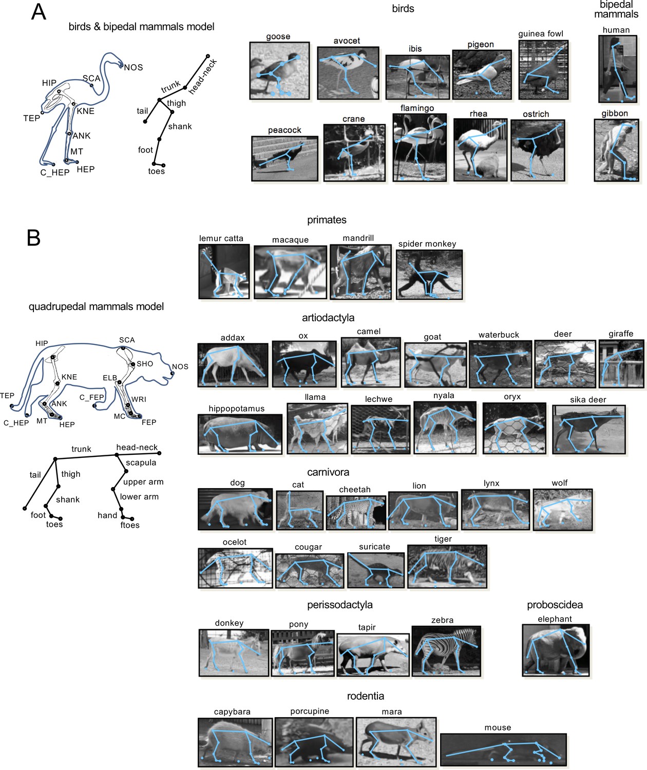
Anatomical landmarks and segments used for the kinematic model of bipedal.
(A) and quadrupedal (B) locomotion superimposed on a bird and mammal skeleton (left panels) and extracted video frames (right panels) of the recorded animals. For the kinematic data digitized from Fischer et al. (2002) (animals marked by asterisks in Table 1), the same definition of elevation angles was used.
Figure 2—figure supplement 2
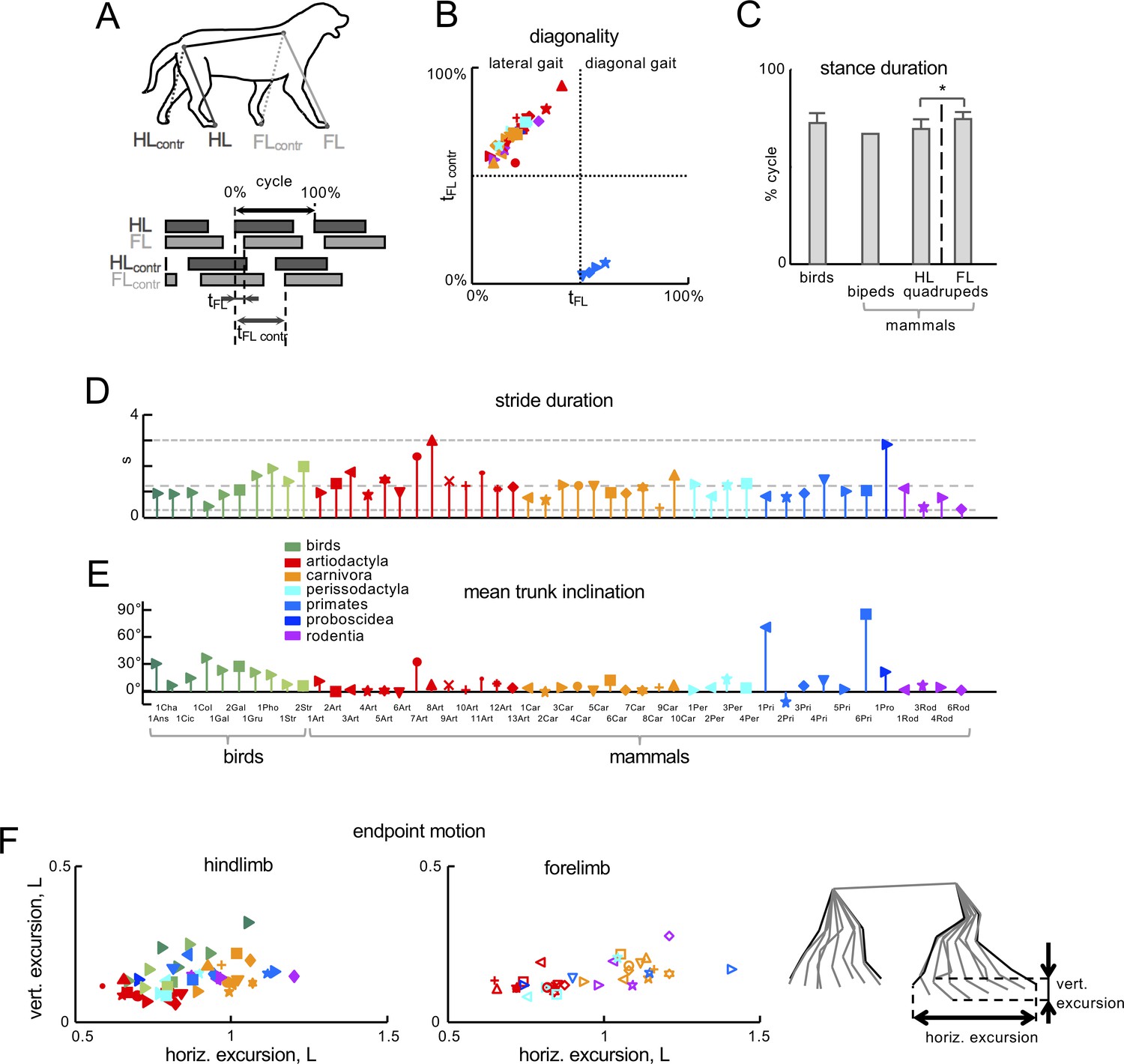
General gait parameters.
(A) Schematic drawing of a walking dog with stick diagram indicating the distal points analyzed and limb contact pattern on the bottom. HL, FL refer to hindlimb and forelimb facing the recording camera, while HLcontr, FLcontr indicate the contralateral ones. Grey bars indicate the period of time in which each foot is in contact with the ground during the stride. (B) Mean FL phase lag (tFL) values plotted versus contralateral FL values (tFLcontr) for all animals. The phase lag was computed as the relative timing (tFL, tFLcontr) of the FL cycle onset with respect to HL, expressed as a percentage of the gait cycle (see panel A). (C) Relative duration of the stance phase (mean +SD across animals). Asterisk indicates significant differences between HL and FL of mammals (p<0.001). (D) Stride duration. (E) Mean trunk inclination during walking with respect to the horizon. (F) Endpoint motion. The stick diagram of a single stride of a walking dog illustrates limb segment movements relative to hip (for HL) and scapula (for FL). Bottom plots show vertical vs. horizontal limb endpoint excursions, normalized to the limb length (L equals to the sum of the lengths of thigh, shank, and foot segments). The data in panels B-F do not include animals marked by asterisks in Table 1 (since this information is missing in Fischer et al., 2002). Animals are labeled as in Table 1 and different colors and markers refer to different taxonomic orders and species, respectively. Source files are available in the SourceData2-Figure 2—figure supplement 2—souce data 1.zip file.
-
Figure 2—figure supplement 2—source data 1
General gait parameters.
- https://doi.org/10.7554/eLife.38190.009
Figure 3 with 2 supplements

Planar covariation of limb segment angular motion.
(A) Ensemble-averaged (±SD across strides) limb segment elevation angles plotted vs.normalized gait cycle and three-dimensional gait loops with corresponding interpolation planes on the bottom are shown for one bird (avocet) and one mammal (elephant). For FL, planar covariation was examined using different tri-segmental FL models: FLupp – ‘scapula–upper arm–lower arm’ and FLlow – 'upper arm–lower arm–hand’. Note roughly similar orientation of the covariation plane between these two models of FL and different orientation compared to the HL model. (B) Planarity index expressed in percent of variance (PV) accounted for by the third principal component (PC) for HL and FL of animals (PV3 = 0 for ideal planarity). Source files are available in the SourceData3-Figure3.zip file.
-
Figure 3—source data 1
Planar covariation of limb segment motion.
- https://doi.org/10.7554/eLife.38190.016
Figure 3—figure supplement 1
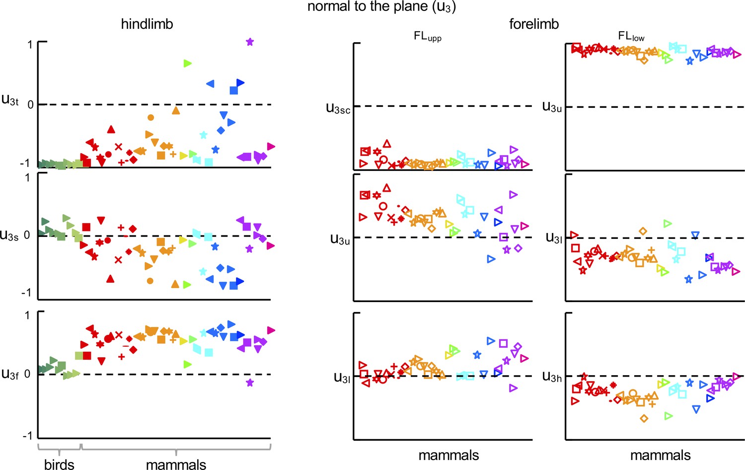
Direction cosines of the normal to the covariation plane (the dot product of u3 with the unit vector along each of the three axes: u3t, u3s, u3f for HL and u3sc, u3u, u3l and u3u, u3l, u3h for FLupp and FLlow, respectively) for all animals.
Source files are available in the SourceData3-Figure 3—figure supplement 1—souce data 1.zip file.
-
Figure 3—figure supplement 1—source data 1
Direction cosine of the normal to the covariation plane.
- https://doi.org/10.7554/eLife.38190.013
Figure 3—figure supplement 2
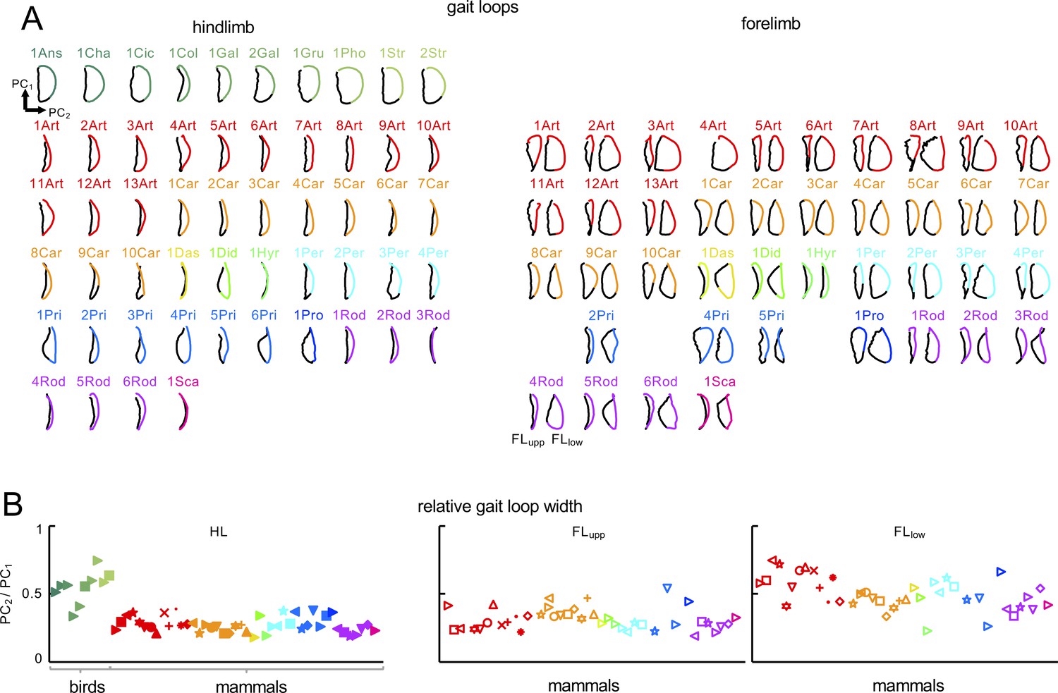
Gait loops in birds and mammals.
(A) Bi-dimensional view of gait loops (Figure 3A) for each animal, projected on the covariation plane. Each loop is rotated so that the first and second principal components are aligned with the vertical and horizontal axes of the figure. Paths progress in time in the counter clockwise direction, touchdown and lift-off events (stance phase in black) corresponding to the top and bottom of the loops, respectively. Animal are labeled as in Table 1. For FL, gait loops for the FLupp and FLlow tri-segmental models are shown. (B) Relative gait loop width estimated as the amplitude (peak-to-peak) of PC2 relative to PC1. Note that the FLlow loop is wider than the HL loop for mammals and the HL loop is wider for birds than for mammals. Source files are available in the SourceData3-Figure 3—figure supplement 2—souce data 1.zip file.
-
Figure 3—figure supplement 2—source data 1
Gait loops.
- https://doi.org/10.7554/eLife.38190.015
Figure 4 with 1 supplement

Orientation (u3 vector) of the covariation plane for the HL (A) and FL (B) segment elevation angles.
For FL, the normal to the plane for both FLupp and FLlow tri-segmental models are shown. Top panels: spatial distribution of the normal (u3) to the covariation plane in all animals. Each vector u3 yields one point corresponding to the projection of the plane normal onto the unit sphere, the axes of which are the direction cosines with the axes of segment elevation angles (u3t, u3s, u3f). Positive direction of the semi-axes is indicated by arrow. Lower panels: u3 vectors for different animals lay on the plane (perpendicular to the averaged u1 vector across animals), α - angle of rotation of u3 on this plane (α = 0 corresponds to the projection of the shank, upper arm and lower arm semi-axes on that plane for HL, FLupp and FLlow, respectively). Animals are labeled as in Table 1 and different colors and markers refer to different taxonomic orders and species, respectively. Note a higher data dispersion for HL compared to FL across animals. Source files are available in the SourceData4-Figure4.zip file.
-
Figure 4—source data 1
Orientation of the covariation plane.
- https://doi.org/10.7554/eLife.38190.020
Figure 4—figure supplement 1
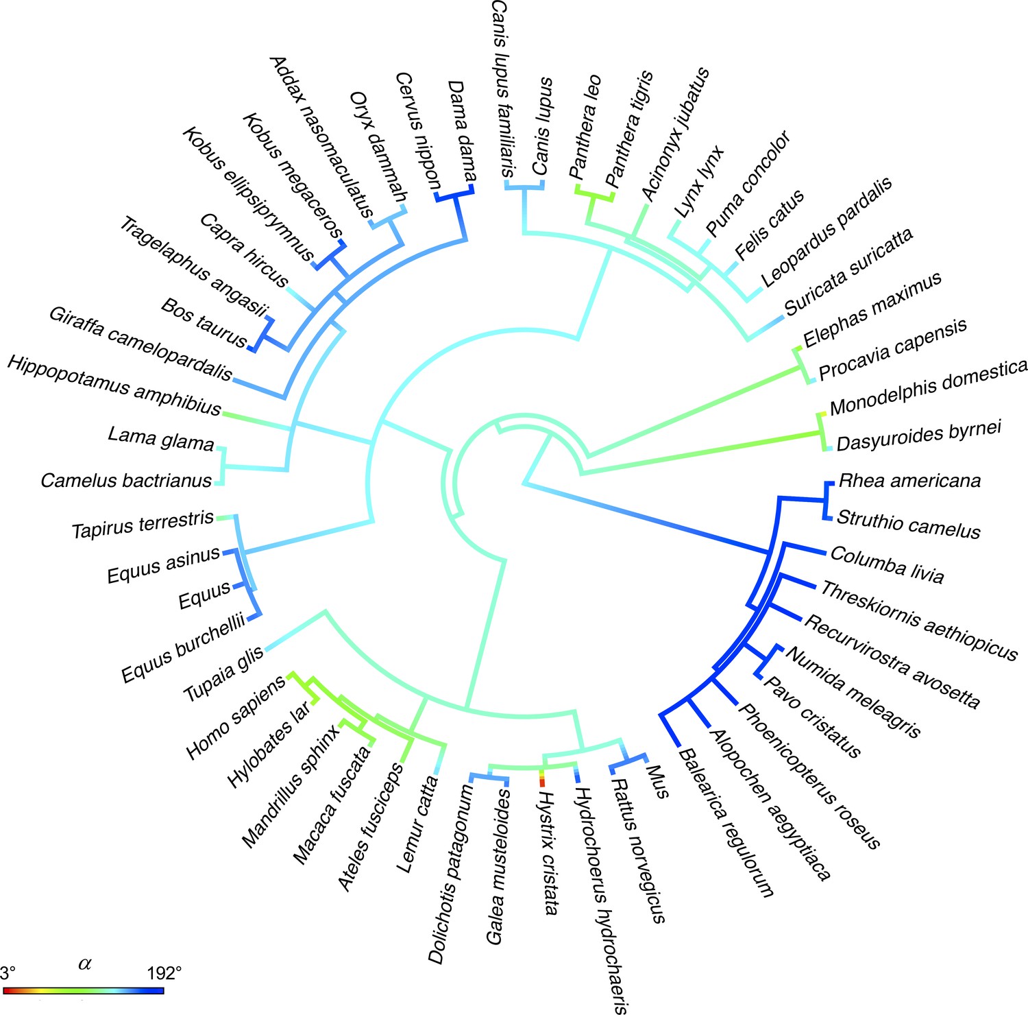
Reconstructed ancestral trait values of α for HL on a phylogeny.
Reconstructed ancestral states for a continuous trait, that is the angle α for HL (angle of rotation of u3, Figure 4A), are plotted in a color scale with gradient projection onto the phylogenetic tree. Note that close relatives are not more similar than distant ones (except for birds), as also shown by the low phylogenetic signal (K = 0.1, see main text). Source files are available in the SourceData4-Figure 4—figure supplement 1—souce data 1.zip file.
-
Figure 4—figure supplement 1—source data 1
Reconstructed ancestral trait values.
- https://doi.org/10.7554/eLife.38190.019
Figure 5
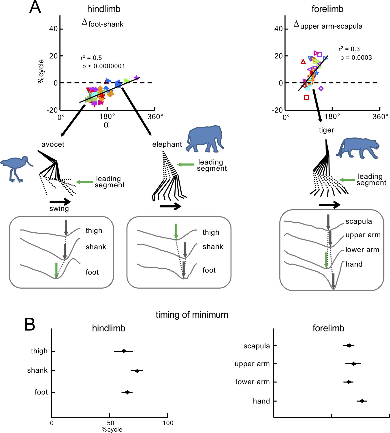
Significant correlations between the orientation of the covariation plane and the phase shifts between elevation angles.
(A) Relationships between Δfoot-shank, Δupper arm-scapula (the differences between the timing of minima of elevation angles) and orientation of the u3 vector (α angle in Figure 4). Linear regressions are also displayed with corresponding r2 and p-values. On the bottom of panel A: examples of the limb segment elevation angles for HL of avocet and elephant, and FL of tiger. The sequence of minima is indicated by arrows. The leading segment, which corresponds to the first minimum and initiates the swing phase (green arrow) is highlighted by dotted lines in the stick diagrams. (B) Timing of minima (±SD) of the limb segment elevation angles of HL and FL of all animals expressed in percent of gait cycle. Source files are available in the SourceData5-Figure5.zip file.
-
Figure 5—source data 1
Significant correlations between the orientation of the covariation plane and the phase shifts.
- https://doi.org/10.7554/eLife.38190.022
Figure 6
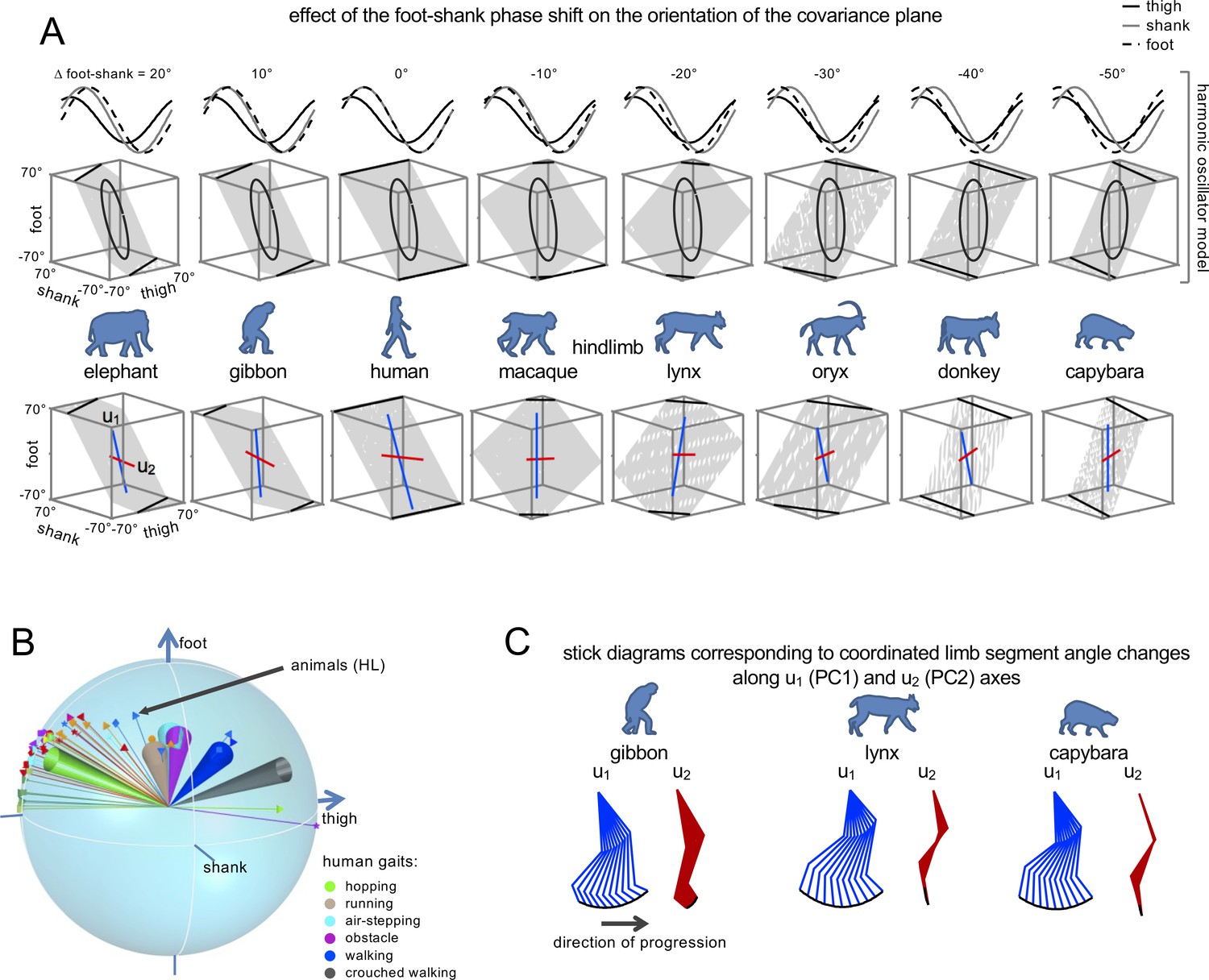
Inter-segmental coordination patterns.
(A) Effect of the foot-shank phase shift on the orientation of the covariation plane. Upper panels: Harmonic oscillator model of Barliya et al. (2009) approximating the three segment elevation angles by sinusoidal waveforms with specific phase and amplitude. By changing the phase of the foot segment waveform relative to the shank segment from 20° to −50° (corresponding to the same range of Δfoot-shank in Figure 5A), the covariation plane rotates similarly to the actual plane rotation across animals (lower panels, blue and red lines indicate the orientation of u1 and u2 vectors, respectively). (B) Similar plane of rotation of the u3 vector across animals (HL, Figure 4A) and different human gaits (indicated by colored confidence cones, the data are redrawn from Figure 2B in Ivanenko et al., 2007). (C) Examples of stick diagrams corresponding to the coordinated limb segment angle changes along u1 (PC1) and u2 (PC2) axes (indicated by color lines in panel A, bottom plots). Note that PC1 reproduces the whole limb orientation changes while PC2 is mainly associated with changes in the limb length. Source files are available in the SourceData6-Figure6.zip file.
-
Figure 6—source data 1
Inter-segmental coordination patterns.
- https://doi.org/10.7554/eLife.38190.024
Tables
Table 1
Analyzed animals.
The table shows the taxonomic classification with class, order and scientific name as reported in http://tolweb.org/tree/, http://www.arkive.org/, https://animaldiversity.org/, and the English name. Animals are sorted in the following order: birds - anseriformes, charadriformes, ciconiformes, columbiformes, galliformes, gruiformes, phoenicopteriformes, struthioniformes - and mammals - artiodactyla, carnivora, dasyuromorphia, didelphimorphia, hyracoidea, perissodactyla, primates, proboscidae, rodentia, scandentia. The locations where the animals were recorded are labeled by capital letters: F - Falconara zoo (Falconara, Italy); N - Iacchelli Farm (Nemi, Italy); R - Zoo of Rome (Rome, Italy); J - Nara City (Nara, Japan); LF – Fischer laboratory (Fischer et al., 2002); LA – Akay laboratory (Akay et al., 2014); LR – our laboratory (Rome, Italy). Next, we identify each species with a serial number and the first three letters of the corresponding taxonomic order, we report the number of analyzed animals, the typical body weight of adults (data from the literature), the mean speed for the recorded strides, the approximate dimensionless speed (Froude number, Fr), and the total number of analyzed strides for hindlimbs and forelimbs. For humans, we recorded both overground walking in one subject and treadmill walking (at 5 km/hr) in five subjects (data pooled together). For mice, video recordings were used from a previously published study (Movie S1 in Akay et al., 2014), while the kinematic data of the six mammals marked by asterisks are derived from Fischer et al. (2002). In the latter case, the number of averaged strides varied: at least 15, but up to 300 step cycles were averaged.
| Order | Animals | Location | Label | N of animals | Typical weight (kg) | V (m/s) | Fr | N of strides | ||
|---|---|---|---|---|---|---|---|---|---|---|
| HL | FL | |||||||||
| Birds | Anseriformes | Goose (Alopochen aegyptiaca) | F | 1Ans | 2 | 1.9 | 0.66 | 0.12 | 9 | - |
| Charadriiformes | Avocet (Recurvirostra avosetta) | F | 1Cha | 6 | 0.3 | 0.43 | 0.06 | 8 | - | |
| Ciconiiformes | Ibis (Threskiornis aethiopicus) | F | 1Cic | 3 | 15 | 0.54 | 0.09 | 5 | - | |
| Columbiformes | Pigeon (Columba livia) | N | 1Col | 3 | 0.4 | 0.72 | 0.32 | 7 | - | |
| Galliformes | Guinea fowl (Numida meleagris) | N | 1 Gal | 5 | 1.3 | 0.48 | 0.06 | 11 | - | |
| Peacock (Pavo cristatus) | R | 2 Gal | 4 | 4.4 | 0.60 | 0.06 | 11 | - | ||
| Gruiformes | Crane (Balearica regulorum) | F | 1Gru | 2 | 3.5 | 0.39 | 0.04 | 5 | - | |
| Phoenicopteriformes | Flamingo (Phoenicopterus roseus) | F | 1Pho | 6 | 2.5 | 0.36 | 0.02 | 11 | - | |
| Struthioniformes | Rhea (Rhea americana) | R | 1Str | 5 | 25 | 0.56 | 0.04 | 11 | - | |
| Ostrich (Struthio camelus) | F | 2Str | 6 | 110 | 0.57 | 0.03 | 10 | - | ||
| Mammals | Artiodactyla | Addax (Addax nasomaculatus) | R | 1Art | 1 | 93 | 1.07 | 0.12 | 2 | 2 |
| Ox (Bos taurus) | F | 2Art | 2 | 755 | 0.71 | 0.07 | 6 | 5 | ||
| Camel (Camelus bactrianus) | F | 3Art | 2 | 475 | 1.08 | 0.08 | 10 | 7 | ||
| Goat (Capra hircus) | F | 4Art | 2 | 45 | 1.17 | 0.16 | 3 | 2 | ||
| Waterbuck (Kobus ellipsiprymnus) | F | 5Art | 2 | 215 | 0.82 | 0.07 | 8 | 7 | ||
| Deer (Dama dama) | F | 6Art | 4 | 56 | 0.95 | 0.12 | 10 | 7 | ||
| Giraffe (Giraffa camelopardalis) | F,R | 7Art | 4 | 1560 | 1.21 | 0.06 | 9 | 10 | ||
| Hippopotamus (Hippopotamus amphibious) | F | 8Art | 1 | 2250 | 0.37 | 0.01 | 7 | 1 | ||
| Llama (Lama glama) | F | 9Art | 3 | 143 | 0.53 | 0.04 | 5 | 5 | ||
| Lechwe (Kobus megaceros) | R | 10Art | 4 | 175 | 0.79 | 0.07 | 7 | 5 | ||
| Nyala (Tragelaphus angasii) | F | 11Art | 3 | 91 | 0.57 | 0.03 | 5 | 4 | ||
| Oryx (Oryx dammah) | F | 12Art | 2 | 190 | 0.97 | 0.12 | 10 | 10 | ||
| Sika deer (Cervus nippon) | J | 13Art | 3 | 63 | 0.78 | 0.09 | 6 | 6 | ||
| Carnivora | Dog (Canis lupus familiaris) | R | 1Car | 6 | 35 | 1.06 | 0.24 | 35 | 36 | |
| Cat (Felis catus) | R | 2Car | 2 | 8 | 1.00 | 0.27 | 6 | 5 | ||
| Cheetah (Acinonyx jubatus) | F | 3Car | 2 | 50 | 0.87 | 0.10 | 10 | 9 | ||
| Lion (Panthera leo) | F | 4Car | 1 | 130 | 1.32 | 0.17 | 10 | 10 | ||
| Lynx (Lynx lynx) | F | 5Car | 1 | 20 | 0.81 | 0.11 | 10 | 10 | ||
| Wolf (Canis lupus) | F | 6Car | 1 | 40 | 1.05 | 0.20 | 6 | 6 | ||
| | | Ocelot (Leopardus pardalis) | F | 7Car | 1 | 13 | 0.78 | 0.15 | 9 | 9 |
| Cougar (Puma concolor) | F | 8Car | 2 | 62 | 1.05 | 0.18 | 10 | 10 | ||
| Suricate (Suricata suricatta) | F | 9Car | 6 | 0.7 | 0.63 | 0.29 | 10 | 8 | ||
| Tiger (Panthera tigris) | F | 10Car | 2 | 257 | 1.22 | 0.13 | 8 | 8 | ||
| Dasyuromorphia | Kowari (Dasyuroides byrnei*) | LF | 1Das | 2 | 0.145 | * | * | * | * | |
| Didelphimorphia | Short-tailed opossum (Monodelphis domestica*) | LF | 1Did | 2 | 0.092 | * | * | * | * | |
| Hyracoidea | Rock hyrax(Procavia capensis*) | LF | 1Hyr | 2 | 1.2 | * | * | * | * | |
| Perissodactyla | Donkey (Equus asinus) | F | 1Per | 2 | 203 | 0.81 | 0.07 | 16 | 12 | |
| Pony (Equus) | F | 2Per | 1 | 50 | 1.02 | 0.16 | 11 | 11 | ||
| Tapir (Tapirus terrestris) | R | 3Per | 2 | 200 | 0.99 | 0.12 | 2 | 1 | ||
| Zebra (Equus burchellii) | F | 4Per | 4 | 310 | 1.18 | 0.12 | 11 | 11 | ||
| Primates | Gibbon (Hylobates lar) | F | 1Pri | 3 | 5 | 1.03 | 0.23 | 6 | - | |
| Lemur catta (Lemur catta) | F,R | 2Pri | 7 | 3.9 | 0.66 | 0.14 | 10 | 3 | ||
| Macaque (Macaca fuscata) | R | 3Pri | 2 | 9.8 | 0.86 | 0.14 | 2 | 0 | ||
| Mandrill (Mandrillus sphinx) | R | 4Pri | 3 | 18 | 0.55 | 0.05 | 7 | 4 | ||
| Spider monkey (Ateles fusciceps) | F | 5Pri | 3 | 9 | 0.75 | 0.13 | 3 | 2 | ||
| Human (Homo sapiens) | LR | 6Pri | 6 | 68 | 1.46 | 0.27 | 67 | - | ||
| Proboscidea | Elephant (Elephas maximus) | R | 1Pro | 1 | 4050 | 1.24 | 0.07 | 6 | 6 | |
| Rodentia | Capybara (Hydrochoerus hydrochaeris) | F | 1Rod | 4 | 51 | 0.68 | 0.10 | 5 | 3 | |
| Cavy (Galea musteloides*) | LF | 2Rod | 2 | 0.3 | * | * | * | * | ||
| Porcupine (Hystrix cristata) | F | 3Rod | 2 | 20 | 1.17 | 0.50 | 4 | 3 | ||
| Mara (Dolichotis patagonum) | F | 4Rod | 3 | 8.1 | 0.82 | 0.18 | 9 | 9 | ||
| Rat (Rattus norvegicus*) | LF | 5Rod | 3 | 0.35 | * | * | * | * | ||
| Mouse (Mus) | LA | 6Rod | 1 | 0.03 | 0.52 | 0.34 | 3 | 3 | ||
| Scandentia | Common treeshrew (Tupaia glis*) | LF | 1Sca | 2 | 0.18 | * | * | * | * | |
Additional files
-
Transparent reporting form
- https://doi.org/10.7554/eLife.38190.025
Download links
A two-part list of links to download the article, or parts of the article, in various formats.
Downloads (link to download the article as PDF)
Open citations (links to open the citations from this article in various online reference manager services)
Cite this article (links to download the citations from this article in formats compatible with various reference manager tools)
A kinematic synergy for terrestrial locomotion shared by mammals and birds
eLife 7:e38190.
https://doi.org/10.7554/eLife.38190


