FluoEM, virtual labeling of axons in three-dimensional electron microscopy data for long-range connectomics
- Max Planck Institute for Brain Research, Germany
- Radboud University, Netherlands
Figures
Figure 1

FluoEM applications and concept.
(a) Most local circuits in mammalian brains can be mapped densely by modern 3D EM (gray neurons), but the source of a majority of the relevant input axons remain unidentified (colored), because the projections arise from distal brain regions (see sketch on the left). Examples show upper layers of cortex, Amygdala and Striatum with dominant input from other cortices (Cx), Thalamus (Thal.), Hippocampus (HC), Substantia Nigra (SNi). Deciphering the connectomic logic of these inputs within a densely imaged neuronal circuit requires parallel axonal labels in a single EM experiment. Mapping color-encoded information on multiple axonal origins from LM data into 3D EM data useable for connectomic reconstruction in mammalian nervous tissue is the goal of the presented method. (b) A brain tissue sample containing fluorescently labeled axons is volume imaged first using confocal laser scanning microscopy (LM) and then using 3D electron microscopy (EM). The fluorescently labeled axons (red and green) contained in the LM dataset are then matched to the corresponding axons in the EM dataset (black and white) solely based on structural constraints (see b-d), without chemical label conversion or artificial fiducial marks. (c) Coarse LM-EM volume registration based on intrinsic fiducials such as blood vessels (blue) and somata (yellow) can be routinely achieved at a registration precision of about 5 –10 µm (Bock et al., 2011; Briggman et al., 2011). (d) The path length over which fluorescently labeled axons (green and red) in a volume LM dataset are clearly reconstructable depends mostly on the labeling density in the respective fluorescence channel. Blue, blood vessels (B.v.). (e) Axons (grey) traversing a common bounding box (blue) of extent become increasingly distinguishable with increasing distance from the common origin. After a distance , a given axonal trajectory is unique, that is no other axon from the center bounding box is still closer than . Since 3D EM allows the reconstruction of all axons traversing a given bounding box, can be determined (see Figure 2). If axons can be reconstructed at the LM level for a path length (c) that is similar to or larger than the typical axonal uniqueness length (d), the FluoEM approach can in principle be successful.
Figure 2 with 1 supplement
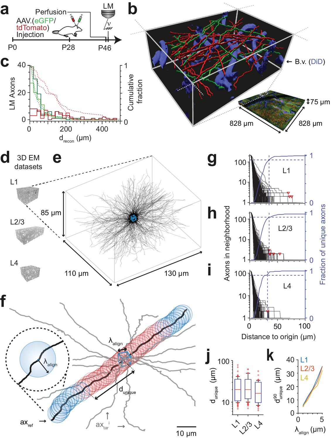
FluoEM proof-of-principle measurements.
(a–c) Measurement of the length over which axons in LM fluorescence data are faithfully reconstructable (see Fig. 1d). (a) Experimental timeline: Injection of a fluorescent-protein (FP) expressing adeno-associated virus at postnatal day 28 (AAV.eGFP into M1 cortex, AAV.tdTomato into S2 cortex of a wild-type C57BL/6j mouse); transcardial perfusion, fixation, sample extraction from cortical L1 at postnatal day 46 followed by confocal volume imaging. (b) Rendering of a subvolume of the three-channel confocal image stack showing axonal long-range projections from M1 cortex (green), S2 cortex (red) as well as stained blood vessels (blue). (c) Histogram of the reconstructable pathlength () for the fluorescently stained long-range axons (red, green) in the example LM dataset (b) based on two independent expert annotations (light and dark colors; median of 28 µm and 33 µm (green channel, n = 115 and 88) and 88 µm and 107 µm (red channel, n = 56 and 47) for the two annotators, respectively). Dashed lines: cumulative axon fraction per annotator and channel. Note that annotators were explicitly asked to stop reconstructions whenever any ambiguity or uncertainty occurred, thus biasing these reconstructions to shorter length. (d–k), EM-based measurements of the length over which the trajectory of axons becomes unique in several cortical layers. (d) Renderings of three 3D EM datasets in layers 1, 2/3 and 4 of mouse cortex. (e) Skeleton reconstructions in the L1 3D EM dataset of all 220 axons (black) that traversed a center bounding box (blue) of edge length = 5 µm. (f) Determination of the uniqueness length for a given axon (black) by counting the number of other axons (gray) that were within the same seeding volume (blue box) and remain within a distance of no more than from the reference axon for increasing distances d from the center box. was defined as the Euclidean distance from the center box at which no other axon persistently was at less than distance from the reference axon (red: at least one neighboring axon, blue: no more neighboring axon). (g) Axonal uniqueness length in cortical L1 for all n = 220 axons from the center bounding box (see e). Number of neighboring axons for each axon (black) and the combined fraction of unique axons (blue) over Euclidean distance from the bounding box center. Note that at = 35 µm the trajectory of 90% of all axons has become unique (dashed blue line). For three of 220 axons, one or two other axons remained in proximity within the dataset (red triangles). (h,i) Axonal uniqueness length in two additional 3D EM datasets from L2/3 (h, n = 207 axons) and L4 (i, n = 128 axons), labels as as in g. (j) Box plot of uniqueness length per axon for cortical layers 1-4 (from g-i). Boxes indicate (10th, 90th)-percentiles, whiskers indicate (5th, 95th)-percentiles, red crosses indicate outliers. (k) Effect of the coarse alignment precision on axonal uniqueness length (resampled for smaller = 1, 2, 3, 4 µm, see Materials and methods).
-
Figure 2—source data 1
Axonal uniqueness analysis for cortical layer 1 (Figure 2g).
- https://doi.org/10.7554/eLife.38976.005
-
Figure 2—source data 2
Axonal uniqueness analysis for cortical layer 2/3 (Figure 2h).
- https://doi.org/10.7554/eLife.38976.006
-
Figure 2—source data 3
Axonal uniqueness analysis for cortical layer 4 (Figure 2i).
- https://doi.org/10.7554/eLife.38976.007
-
Figure 2—source data 4
Axonal uniqueness summary boxplot (Figure 2j).
- https://doi.org/10.7554/eLife.38976.008
-
Figure 2—source data 5
Axonal uniqueness dependence on alignment error (Figure 2k).
- https://doi.org/10.7554/eLife.38976.009
Figure 2—figure supplement 1

Axonal uniqueness length for different cortical layers corrected for numbers of contained axons.
Bars indicate mean (error bars: s.d.) of the bootstrapped L1 and L2/3 axon bounding box samples (n = 128 out of L1: n = 220, L2/3: n = 207 axons per random subsample, n = 30 draws). For L4 (n = 128 axons contained in bounding box sample) bar indicates . Statistical tests do not indicate a significant axon uniqueness length difference between the bootstrapped L1 and L2/3 distributions and the L4 sample mean (L1: p = 0.54; L2/3: p = 0.14, see Materials and methods: Statistical tests).
Figure 3
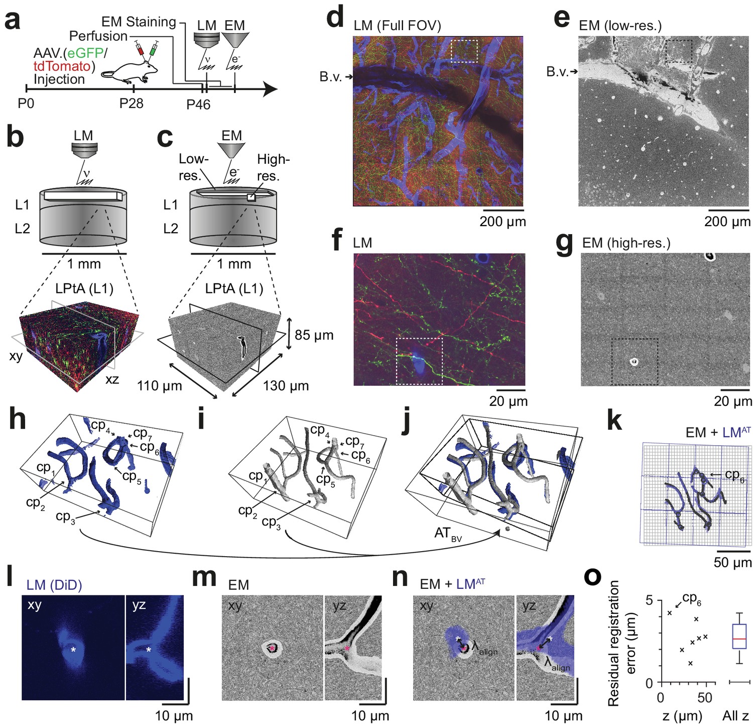
Coarse LM-EM registration.
(a) Experimental timeline for FluoEM experiment (continued from Fig. 2a). After LM imaging was concluded the sample was immediately stained for EM and embedded, followed by 3D EM imaging. (b,c) Sketch of sequentially acquired 3D LM and EM datasets from cortical layer 1 (L1). Fluorescence channels: green (axonal projections from M1 cortex, eGFP); red (axonal projections from S2 cortex, tdTomato); blue (blood vessels, DiD). Volume and voxel size of EM datasets: (1500 x 1000 x 10) µm3 and (700 x 700 x 200) nm3 (low-resolution EM dataset), (130 x 110 x 85) µm3 and (11.24 x 11.24 x 30) nm3 (high-resolution EM dataset). (d,e) Overview images of the LM (d, https://wklink.org/5974) and low-resolution EM (e, https://wklink.org/4610) datasets. Dashed rectangle indicates the position of the high-resolution EM dataset (g, see c for relative positions of datasets). B.v., blood vessel. Note the corresponding pattern of surface vessels in d,e. (f,g) High-resolution images at corresponding locations in LM (f, https://wklink.org/1204) and EM (g, https://wklink.org/5386). Dashed rectangles indicate regions shown in l-n. (h,i), Rendering of blood vessel segmentations in LM (h) and EM (i) and their characteristic bifurcations used as control point pairs (cp1-7) to constrain a coarse affine transformation (ATBV). (j) Overlay of the EM and LMAT blood vessel segmentations registered using ATBV. (k) Registered blood vessels (lines) and control points (circles) overlaid with EM (black) and transformed LM (blue) coordinate grids. (l–n) LM (l) and EM (m) image planes (xy) and reslice (yz) showing an exemplary blood vessel bifurcation (asterisk indicates cp6, see h-k) and the overlay (n) of the affine transformed LM blood vessel segmentation with EM. Arrows indicate registration residual, a measure of the coarse alignment precision . (o) Alignment precision reported as residuals of control point alignment along dataset depth (denoted with z) (mean: 2.7 ± 1.1 µm, median: 2.7 µm) after affine transformation ATBV.
-
Figure 3—source data 1
Blood vessel based affine registration error (Figure 3o).
- https://doi.org/10.7554/eLife.38976.011
Figure 4 with 1 supplement
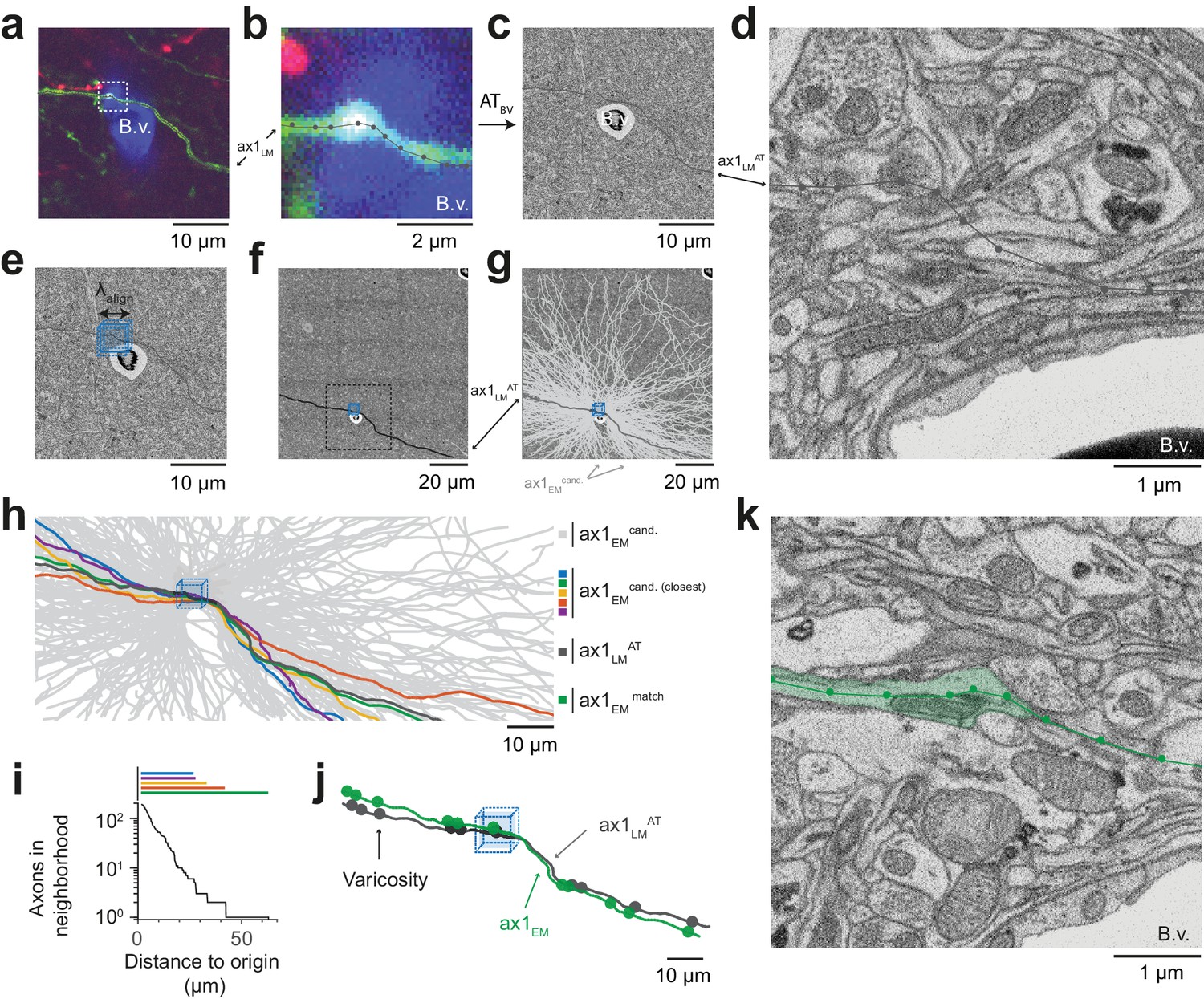
Initial LM-to-EM axon matching.
(a,b) LM image plane showing an axon (green) overlaid with its LM-based skeleton reconstruction (ax1LM, black) and a nearby blood vessel (B.v., blue) bifurcation (a, https://wklink.org/1399). Dashed rectangle, region magnified in (b, https://wklink.org/5406). (c,d) EM image plane showing the blood vessel (B.v.) corresponding to the vessel shown in (a,b) overlaid with the coarse affine transformation (see Figure 3) of the LM-based axon reconstruction ax1LMAT; magnified in d. Note that ax1LMAT does not match the ultrastructural features at high-resolution EM (d) due to the limited precision of ATBV. (e,f), EM plane overlaid with ax1LMAT (as shown in c) with bounding box for dense axon reconstruction (light blue) of edge length = 5 µm; demagnified in f, dashed rectangle denotes region shown in e. (g) Skeleton reconstructions of all n = 193 ax1EM candidates (light grey) traversing the search bounding box (as in e-f), https://wklink.org/5897 (h) Reconstructed ax1EM candidates (light grey) and the transformed fluorescent axon skeleton ax1LMAT (black). Five candidate EM reconstructed axons with the most similar trajectories as ax1LMAT highlighted in different colors. (i) Number of EM-reconstructed axons persistently within the neighborhood of the LM-based template axon ax1LMAT. Note that at a distance of 43 µm from the seed center (e-h), only one possible ax1EM candidate (green) remains. (j) Overlay of ax1LMAT and the most likely ax1EM candidate reconstruction. Axonal varicosities (filled circles) were independently annotated in LM and EM. Note the strong resemblance of the varicosity arrangements indicating that ax1EM is the correctly matched EM equivalent of the LM signal (see Figure 4—figure supplement 1) for statistical analysis). (k) EM plane with overlaid ax1EM skeleton (dark green) and volume annotation of the corresponding EM axon ultrastructure (transparent green), https://wklink.org/3268.
-
Figure 4—source data 1
Axonal uniqueness analysis for initial axon match (Figure 4i).
- https://doi.org/10.7554/eLife.38976.014
Figure 4—figure supplement 1
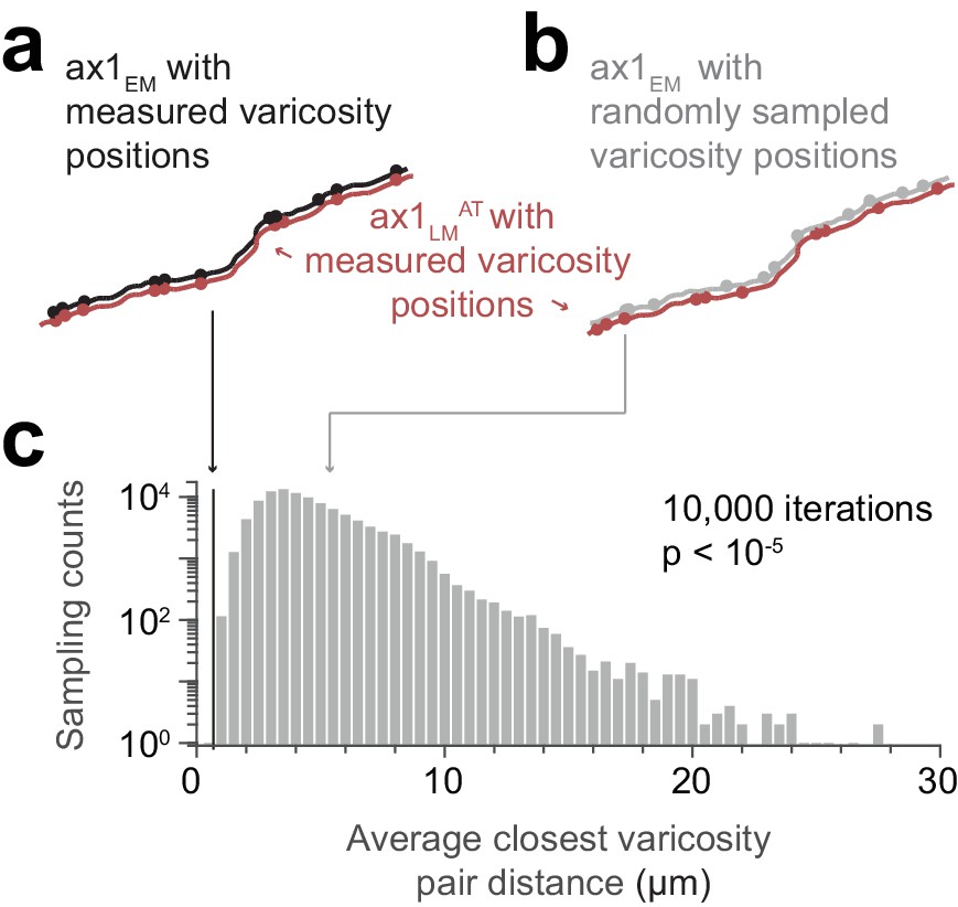
Similarity of matched varicosity patterns between LM and EM.
(a) Independently measured varicosities (red and black circles) highlighted on the skeleton overlay of the initial affine transformed LM axon (ax1LMAT, red) and the EM match candidate (ax1EM, black) (compare Figure 4j). (b) Overlay as in (a) but with ax1EM varicosity positions (grey circles) randomly sampled. (c) Distribution of the average varicosity pair distance between the measured varicosities on ax1LMAT and the respective closest available varicosity on ax1EM for the measured (black line) and randomly sampled (grey histogram bars) positions. The probability of randomly picking (n = 10,000 draws) varicosity positions with an average bouton pair distance as small as or smaller than the measured positions (black line, d = 0.67 µm) is p≤10−5 (see Materials and methods: Statistical tests).
Figure 5 with 1 supplement
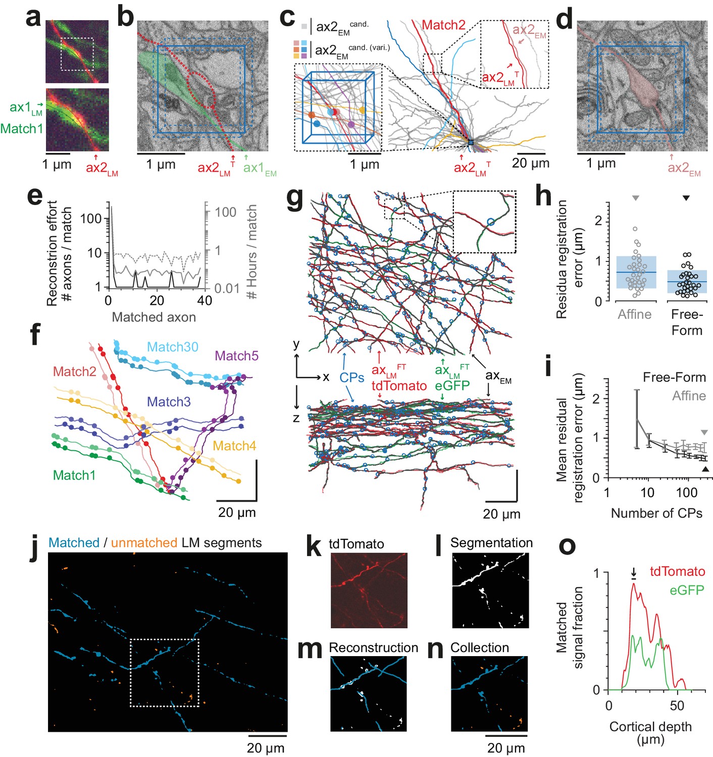
Iterative LM-to-EM axon matching.
(a) Initial axon match ax1LM and nearby axon ax2LM with a varicosity in the proximity, both reconstructed in LM, https://wklink.org/4334. (b) Matched axon ax1EM (light green) and trajectory of axon 2 (ax2LMT) reconstructed at LM and transformed to EM (dashed red line) using a transformation T that was constrained using structural features of the initially matched ax1 (eight control points), https://wklink.org/3305. (c) Search volume sized (2 × 2× 3 ) µm3 (blue box) around the varicosity of ax2LMT (see a-b) containing 34 candidate axons (gray) but only six with candidate varicosities (colored circles). One candidate axon had a similar trajectory as ax2LMT (right inset), identifying it as the correct match (see also varicosity pattern in f). (d) Varicosity in EM of axon ax2EM (red shading, see search template in b), https://wklink.org/3820. (e) Reconstruction effort in terms of number of reconstructed axons (black) and time (grey) required to perform 38 iterative LM-to-EM axon matches. Total effort including full EM-based axon reconstruction and control point placement in LM and EM (dashed grey). (f) Overlay of EM (light colors) and affine transformed LM (dark colors) axon reconstructions of six exemplary matched axon pairs with locations of axonal varicosities (independently reconstructed at LM and EM level, respectively). Note the similarity of axon trajectory and varicosity positions, also for the 30th matched axon. EM axons were offset by 6 µm for visibility, see g for actual overlap quality. (g) Overlay of EM-reconstructed axon skeletons (black) with the matched LM-reconstructed skeletons transformed using a free-form transformation iteratively constrained by control points (CPs, blue circles) obtained from each consecutive axon match (shown transformation used a random subset of 250 (of 284) CPs). (h) Residual registration error of the match shown in g computed as the Euclidean distances || cpEM – cpLMFT || between n = 30 randomly picked CP pairs that had not been previously used to constrain the registration. Sample mean (blue line) and standard deviation (blue shading). (i) Average residual registration error (mean ± s.d., computed as in h) in dependence of the number of randomly chosen control points (CPs) used to constrain the transformation (n = 10 bootstrapped CP sets, each). (j–n) Locally complete LM-to-EM matching of fluorescently labeled axons. One example image plane of LM dataset (at 18 µm depth) shown with EM-matched fluorescence signal fraction (blue) and yet unmatched segments (orange). To compute the matched fluorescence signal fraction, the raw LM data (k) was binarized and segmented (l, see Materials and methods), overlaid with the EM-matched LM axon skeleton reconstructions (m) and only those segments overlapping with skeletons were counted as matched (n). (o) Matched signal fraction (in fraction of matched voxels) over dataset depth. For a range of 17–20 µm depth (black line, arrow), about 90% of the fluorescent voxels were explained by matched EM axons.
-
Figure 5—source data 1
Reconstruction effort (Figure 5e).
- https://doi.org/10.7554/eLife.38976.017
-
Figure 5—source data 2
Axon based affine and free-form registration error (Figure 5h).
- https://doi.org/10.7554/eLife.38976.018
-
Figure 5—source data 3
Averaged axon based affine and free-form registration error depending on control point numbers (Figure 5i).
- https://doi.org/10.7554/eLife.38976.019
-
Figure 5—source data 4
Matched LM signal fraction (Figure 5o).
- https://doi.org/10.7554/eLife.38976.020
Figure 5—figure supplement 1

Deformations of axons in LM vs EM data.
The relative Euclidean displacements resulting from the free-form registration relative to the affine registration along the three cardinal axes are shown as a maximum displacement projection overlaid with 2D projections of the reconstructed axon skeletons. Rows indicate the viewing direction, columns indicate the displacement component color-coded in the heatmaps.
Figure 6
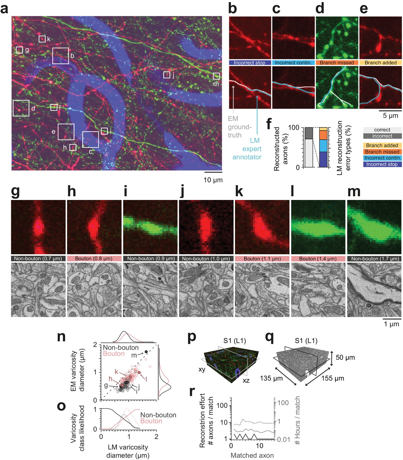
Calibration of axons and synapses in 3D fluorescent data using FluoEM, and reproduction experiment.
(a) Examples of axonal trajectories and axonal varicosities in 3D LM data (Maximum-intensity projection from 42 image planes at 17–35 µm depth; dataset and color code as in Figure 3). (b–f) Post-hoc comparison of axonal reconstructions in LM data and their EM counterparts as identified by FluoEM, which were considered ground truth. Examples of LM reconstruction errors (b–e) and their prevalence (f). Note that while about 70% of axons were correctly reconstructed at the LM level, for about 30%, reconstruction errors such as missed branches or incorrect continuations occurred. Direct links to example locations in the dataset for viewing in webKnossos: b, https://wklink.org/1500 and https://wklink.org/8693; c, https://wklink.org/2441 and https://wklink.org/8447; d, https://wklink.org/5600 and https://wklink.org/4519; e, https://wklink.org/1977 and https://wklink.org/6578. (g–m) Validation of presynaptic bouton detection in fluorescence data: Examples of axonal varicosities imaged using LM (top row) and EM (bottom row). EM was used to determine synaptic (bouton) vs. non-synaptic varicosities. Size of varicosity reported as sphere-equivalent diameter (see Materials and methods). Direct links to example locations in the dataset for viewing in webKnossos: g, https://wklink.org/3721 and https://wklink.org/8170; h, https://wklink.org/6118 and https://wklink.org/7611; i, https://wklink.org/7447 and https://wklink.org/3702; j, https://wklink.org/9694 and https://wklink.org/6772; k, https://wklink.org/4867 and https://wklink.org/0276; l, https://wklink.org/7809 and https://wklink.org/2224; m, https://wklink.org/7269 and https://wklink.org/5832. (n) Relation between the sphere equivalent diameter of axonal varicosities imaged in EM vs. LM for synaptic (red, bouton) and non-synaptic (black) varicosities. (o) Likelihood of varicosities to be synaptic (red) vs. non-synaptic (black) over LM varicosity sphere equivalent diameter, computed from the respective (prevalence-weighted, kernel density estimated) probability densities (dashed, see Materials and methods). (p–r) Second FluoEM experiment from upper cortical L1 in S1 cortex (p: LM dataset subvolume corresponding to (q); q: EM high-res dataset with dimensions) and (r) reconstruction effort for LM-to-EM matching of axons (labels as in Figure 5e).
-
Figure 6—source data 1
Relation between sphere equivalent diameter in LM and EM for synaptic and non-synaptic axonal varicosities (Figure 6n).
- https://doi.org/10.7554/eLife.38976.022
-
Figure 6—source data 2
Sphere diameter dependent synaptic and non-synaptic varicosity likelihood (Figure 6o).
- https://doi.org/10.7554/eLife.38976.023
-
Figure 6—source data 3
Reconstruction effort reproduction experiment (Figure 6r).
- https://doi.org/10.7554/eLife.38976.024
Figure 7
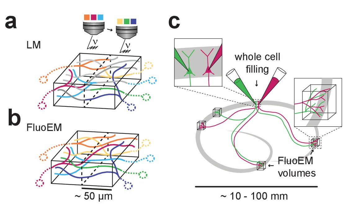
Possible extensions of FluoEM (a,b) Color multiplexing strategy to increase color space without increasing photon dose in FluoEM.
If labeled axons traverse a large volume, then 3D LM imaging can be split into subvolumes of minimal dimension about 50 µm (given by and , see Figure 2) (a), and axon identity can be propagated into the remaining volume via EM reconstruction (b) using the FluoEM approach. (c) Instead of identifying input projections in dense 3D EM by fluorescence labeling, the output connectivity of (multiple) fluorescently labeled neurons in convergent target regions could be studied using FluoEM (see sketch).
Tables
Key resources table
| Reagent type | Designation | Source or reference | Identifiers | Additional information |
|---|---|---|---|---|
| Strain, strain background (Adeno-associated virus) | AAV1.CAG.FLEX.EGFP .WPRE.bGH | Penn Vector core | AllenInstitute854 | Lot: V3807TI-R-DL |
| Strain, strain background (Adeno-associated virus) | AAV1.CAG.FLEX.tdTomato .WPRE.bGH | Penn Vector core | AllenInstitute864 | Lot: V3675TI-Pool |
| Strain, strain background (Adeno-associated virus) | AAV1.CamKII0.4.Cre.SV40 | Penn Vector core | Lot: CS0302 | |
| Chemical compound, drug | 1,1'-Dioctadecyl-3,3,3',3' -Tetramethylindodicarbocyanine | Invitrogen/Thermo Fisher | D7757 | |
| Chemical compound, drug | Paraformaldehyde | Sigma Aldrich/Merck | P6148 | |
| Chemical compound, drug | Glutaraldehyde | Serva | 23116 | |
| Chemical compound, drug | Sodium Cacodylate | Serva | 15540 | |
| Chemical compound, drug | Osmium Tetroxide | Serva | 31253 | |
| Chemical compound, drug | Ferrocyanide (Potassium hexacyanoferrate trihydrate) | Sigma Aldrich/Merck | 60279 | |
| Chemical compound, drug | Thiocarbohydrazide | Sigma Aldrich/Merck | 223220 | |
| Chemical compound, drug | Uranyl acetate | Serva | 77870 | |
| Chemical compound, drug | Lead (II) nitrate | Sigma Aldrich/Merck | 467790 | |
| Chemical compound, drug | L-Aspartic acid | Serva | 14180 | |
| Commercial assay or kit | Spurr low viscosity embedding kit | Sigma Aldrich/Merck | EM0300 |
Additional files
-
Transparent reporting form
- https://doi.org/10.7554/eLife.38976.026
Download links
A two-part list of links to download the article, or parts of the article, in various formats.
Downloads (link to download the article as PDF)
Open citations (links to open the citations from this article in various online reference manager services)
Cite this article (links to download the citations from this article in formats compatible with various reference manager tools)
FluoEM, virtual labeling of axons in three-dimensional electron microscopy data for long-range connectomics
eLife 7:e38976.
https://doi.org/10.7554/eLife.38976


