Entrainment and maintenance of an internal metronome in supplementary motor area
- Institute of Neurobiology, National Autonomous University of Mexico, México
- Massachusetts Institute of Technology, United States
Figures
Figure 1 with 2 supplements
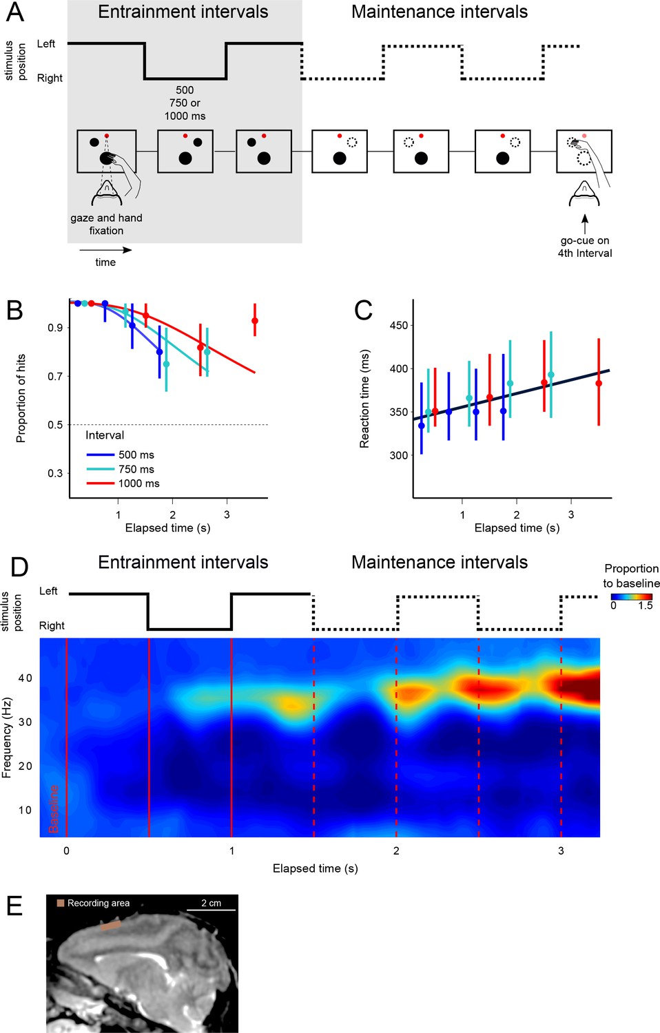
The visual metronome task.
(A) Rhythms of different tempos were defined by a left-right alternating visual stimulus that appeared on a touch screen. While keeping eye and hand fixation, subjects first observed three isochronous entrainment intervals with duration of either 500, 750, or 1000 ms (pseudo-randomly selected on each trial). After the last entrainment interval, the visual stimulus disappeared initiating the maintenance intervals in which subjects had to keep track of the stimulus’ virtual location (left or right, broken lines). A go-cue (extinction of the hand fixation) at the middle of any of the four maintenance intervals prompted the subjects to reach toward the estimated location of the stimulus. It is important to note that this was not an interception task because the left-right switching stopped at the time of the go-cue. Monkeys received a liquid reward when correctly indicating the stimulus location. (B) The proportion of correct responses is plotted as a function of elapsed time during the maintenance intervals. Colors indicate the performance for the three tempos (500, 750, 1000 ms). Performance was significantly above chance (broken line at p=0.5; z-test p<0.001; n = 131 sessions; median ±I.Q.R. over sessions). The decrease in performance as a function of elapsed time is expected from variability of the subjects’ internal timing in the absence of the external visual rhythm. This drop in performance was captured by a model of timing subject to scalar variability (continuous lines). (C) Reaction times to the go-cue increased as a function of elapsed time (n = 131 sessions; median ±I.Q.R. over sessions). Black line indicates a linear regression on the median reaction times. (D) Mean spectrogram across recording sessions and subjects (500 ms interval). The step traces at the top indicate the stimulus position as a function of time, for entrainment and maintenance intervals. Signal amplitude was normalized with respect to a 500 ms baseline period before stimulus presentation. A salient modulation of the LFP signal is observed around the gamma band (30–40 Hz). Gamma activity rhythmically increases in sync with the left-right transitions of the stimulus. Note also the increase in gamma activity as a function of total elapsed time. (E) Recordings were made from the supplementary motor area (SMA). The recoding chamber on monkey 1 (shown) was centered 23 mm anterior to Ear Bar Zero and 4 mm lateral to the midline, on the left hemisphere. The image shows a sagittal plane 2 mm lateral from the middle.
-
Figure 1—source data 1
Source data for the spectrograms.
- https://doi.org/10.7554/eLife.38983.008
Figure 1—figure supplement 1
Behavioral performance and LFP data for each monkey.
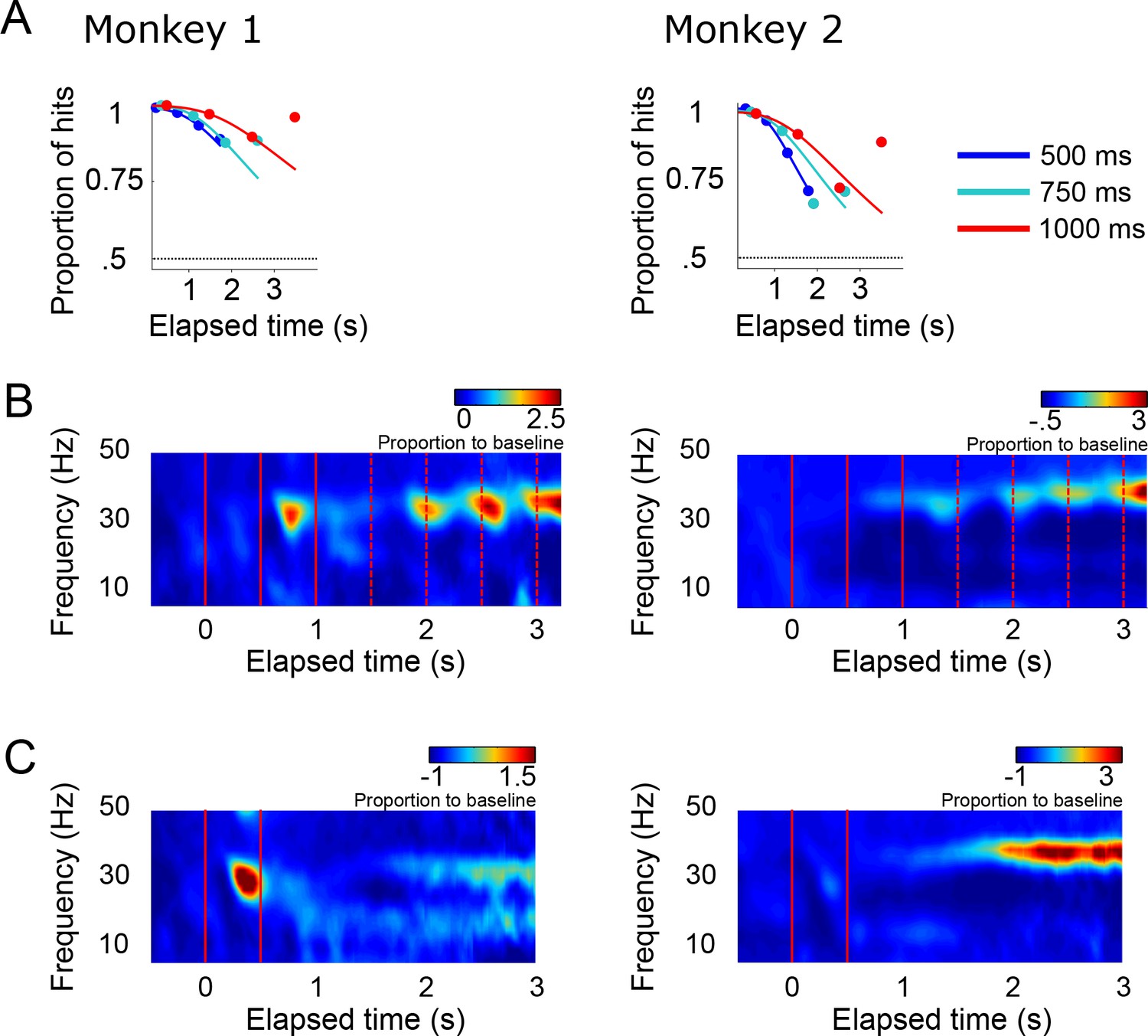
(A) The probability of a correct response is plotted as a function of elapsed time in the maintenance epoch, for each monkey. Same conventions as in Figure 1 of the main text. (B) Mean spectrogram for the LFP recordings of each monkey. Same conventions as in Figure 1. (C) Mean spectrogram for the LFP recordings during the delayed-reach control task. Same conventions as in Figure 5.
-
Figure 1—figure supplement 1—source data 1
Source data for the spectrogram.
- https://doi.org/10.7554/eLife.38983.005
Figure 1—figure supplement 2

Gamma amplitude and reaction times.
(A) Gamma amplitude is positively correlated with reaction time to the go-cue. The residuals of gamma amplitude and reaction time we calculated by subtracting the mean amplitude and reaction time of each of the maintenance intervals (to remove general trends, see main Figure 1). (B) Mean LFP spectrogram aligned to response movement onset. Note how gamma activity decreases before movement initiation, and lower frequencies appear after movement initiation.
-
Figure 1—figure supplement 2—source data 1
Source data for the spectrogram.
- https://doi.org/10.7554/eLife.38983.007
Figure 2
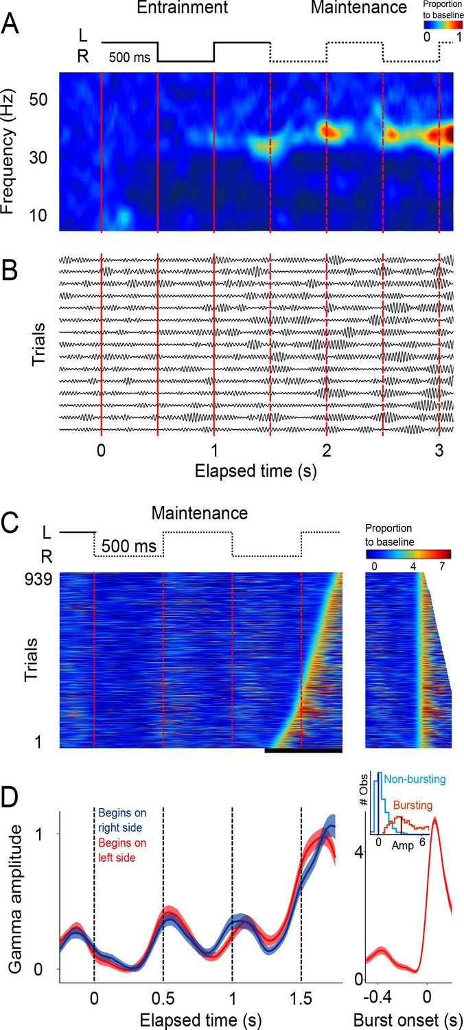
Single trial analysis of the LFP.
(A) Representative spectrogram of 15 single trials (500 ms interval). There is an increase in amplitude at the gamma band (30–40 Hz), particularly salient during maintenance intervals. (B) Single-trials of the LFP signal, band-pass filtered at the 30–40 Hz gamma band. Gamma oscillations are composed of transient bursts during which oscillations increase in amplitude. Note how the bursts tend to occur in sync with left-right transitions of the stimulus and tend increase in amplitude as a function of total elapsed time. (C) Gamma amplitude on each trial is coded by color (939 trials; 500 ms interval, every trial starting on the left is shown, across sessions and subjects). Trials were sorted according to burst onset time within the window marked by the black line at the bottom. The panel on the right shows the last gamma bursts aligned to their onset time. Bursts were defined as the period in which gamma amplitude exceeded the 90th percentile of the amplitude distribution across trials, for at least 100 ms (four cycles of the gamma rhythm). (D) Mean gamma amplitude as a function of elapsed time (n = 131 sessions). Note how the periodic increases in gamma are in sync with the left-right internal rhythm during the maintenance intervals. The panel on the right shows the mean profile of the bursts in the last maintenance interval. The inset shows the distribution of the gamma amplitude during bursting (red distribution) and non-bursting (blue distribution) periods of the trials (dark vertical lines indicate the median burst amplitude for each distribution).
-
Figure 2—source data 1
Source data for the single trial activity.
- https://doi.org/10.7554/eLife.38983.010
Figure 3
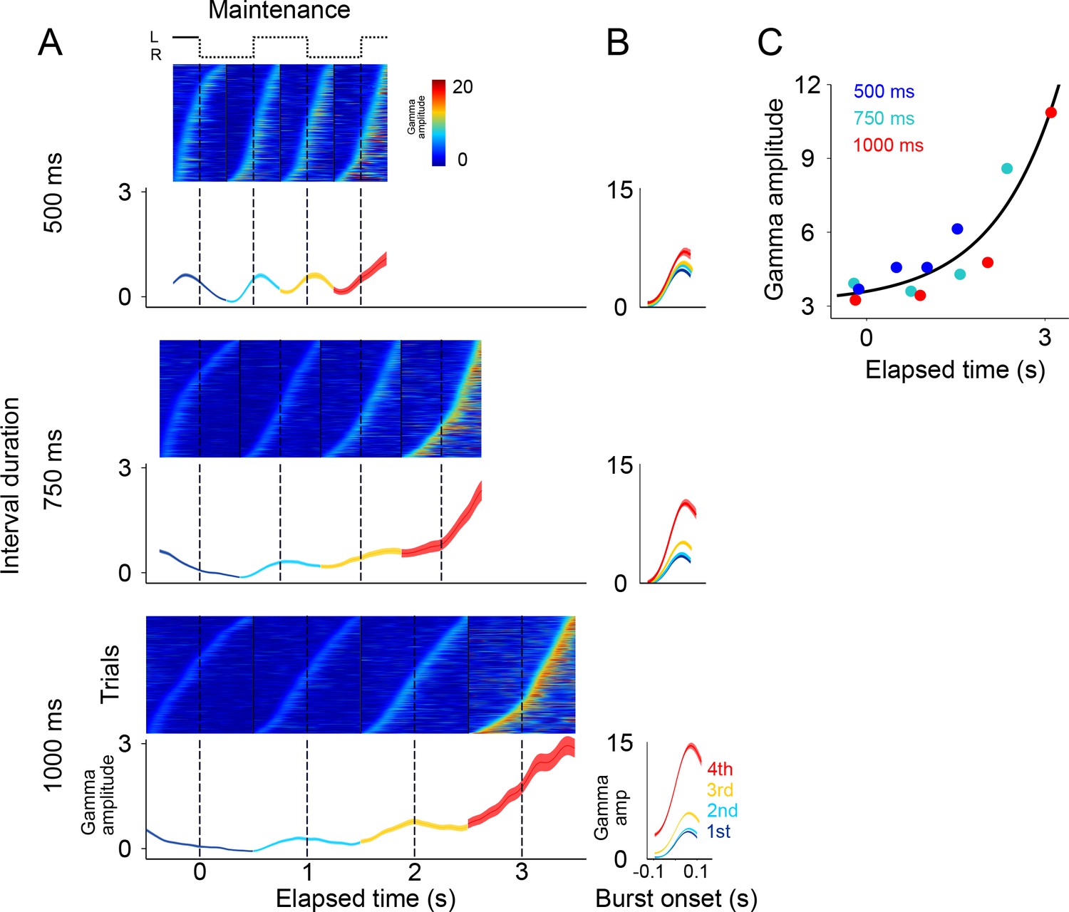
Gamma bursts in maintenance intervals for the three tempos (500, 750, 1000 ms).
(A) For each maintenance interval and tempo, bursts are ordered according to their onset time. Below single trials, mean gamma amplitude is plotted as a function of time (trials starting on the left are shown; 131 sessions; interval duration was pseudo-randomly selected on each trial, but is grouped here for presentation; linewidth denotes s.e. across trials). (B) The temporal profile of gamma bursts is plotted for each stimulus transition (1st, 2nd, 3rd, and 4th, dotted lines in A), and for each interval duration (500, 750, and 1000 ms; top to bottom). The bursts have a stereotyped temporal shape and increase in amplitude after each consecutive transition. (C) Mean amplitude of gamma bursts plotted as a function of elapsed time for the three interval durations (500, 750, and 1000 ms; R2 = 0.86, exponential model).
-
Figure 3—source data 1
Source data for the behavioral performance.
- https://doi.org/10.7554/eLife.38983.012
Figure 4 with 1 supplement

Gamma amplitude in correct and error trials.
(A) Mean gamma amplitude during maintenance intervals, for correct (blue) and error trials (orange) (n = 1400–3000 correct, 260–540 errors; colored area shows s.e. across trials; trials starting on the left are shown, pooled across 131 sessions). The insets on each panel show the periodogram (power spectral density) of correct and error trials (mean across single trials). It can be observed that error trials oscillate at slower frequencies in the 500 ms interval trials, and oscillate at faster frequencies in the 1000 ms trials, as compared to correct responses. (B) Correct and error trials can be classified with increasing accuracy as a function of elapsed time. Two logistic classifiers were used to differentiate between correct and error trials (cross-validated on 50 correct and 50 error trials; n = 100 iterations; colored area shows s.e. across trials). One classifier used a growing window (Cumulative, green line) that incorporated the gamma amplitude data as each trial developed in time. The other classifier used data within a constant length window that slided across each trial (Sliding window, blue line).
-
Figure 4—source data 1
Source data for the spectrograms.
- https://doi.org/10.7554/eLife.38983.015
Figure 4—figure supplement 1

Six-choice version of the metronome task.
(A) The probability of a correct response is plotted as a function of elapsed time for the maintenance intervals. In this version of the task, rhythm tempo was selected randomly from a uniform distribution of 500–1000 ms interval lengths. Trials were split into two groups comprising intervals below and above 750 ms (red and blue lines). Since there are six options for the behavioral response, chance level is at 1/6. (B) Each panel shows the distribution of behavioral responses associated with each maintenance interval. Note how there few errors associated with the first two maintenance intervals. For the 3rd and 4th maintenance intervals, the distribution of responses becomes wider and a pattern of error responses emerges: For the fast intervals (red lines), errors tend to lag behind the correct position. Conversely, for the slow tempos (blue line) errors tend to fall ahead of the correct position. Note how the pattern of errors is not random, but they tend to cluster around the correct response.
Figure 5
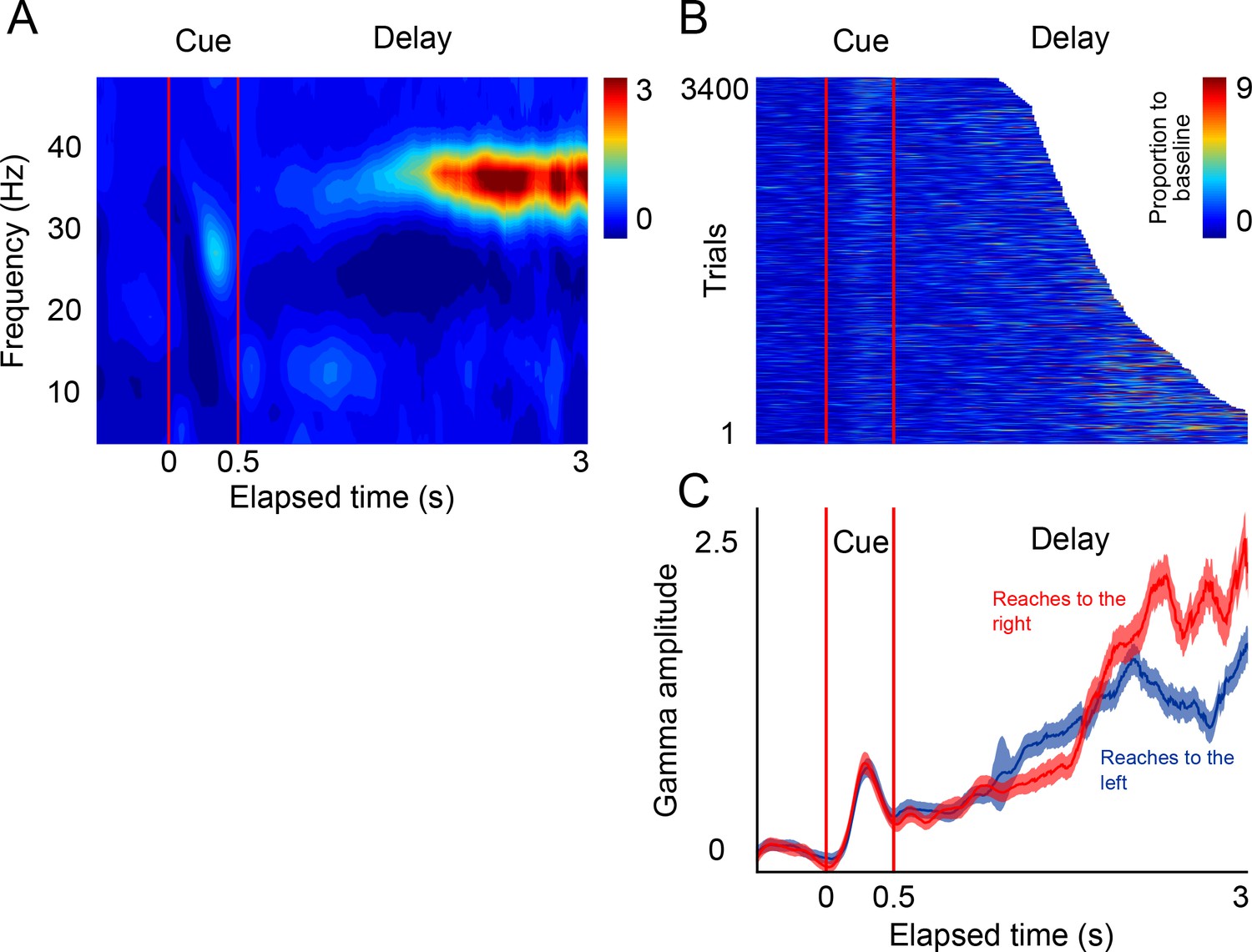
LFP activity in a delayed-reach task.
(A) Mean spectrogram of the LFPs during the delayed-reach task (reaches to the right side of the screen are shown). The stimulus presentation is indicated by the red lines a 0–0.5 s (cue). After the sensory cue, a variable delay between followed (1.2–3 s; exponential distribution). A salient activation of the gamma band during the delay period can be observed (n = 131 sessions). (B) Gamma amplitude across single trials of the delayed-reach task (all trials when cue was presented on right are shown). (C) Mean gamma amplitude plotted as a function of elapsed time. After a brief sensory response, gamma activity increases as a function of elapsed time. Red and blue lines indicate reaches to the right and to the left, respectively.
-
Figure 5—source data 1
Source data for the single trial figures.
- https://doi.org/10.7554/eLife.38983.017
Figure 6
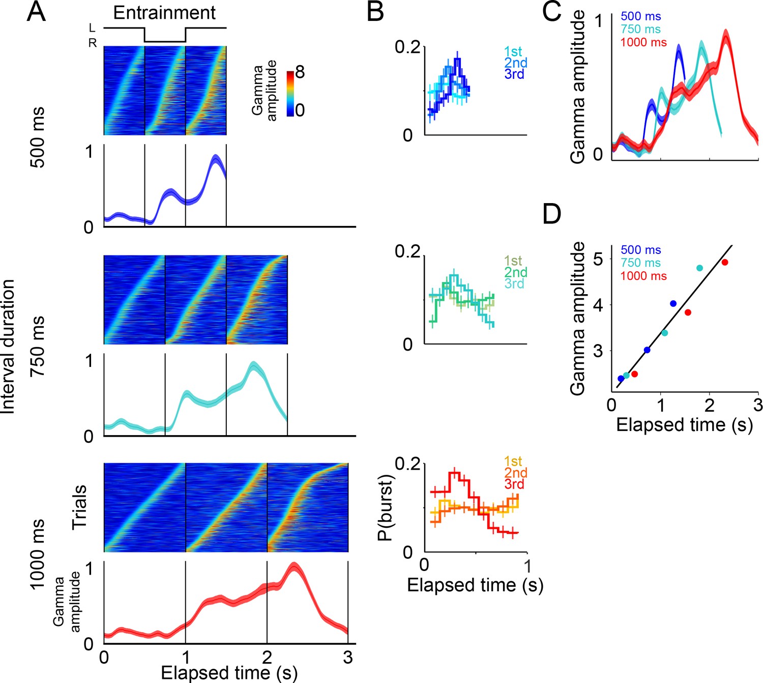
Gamma band activity in entrainment intervals.
(A) Gamma bursts in single trials sorted by their onset time for each entrainment interval, and for each tempo (500, 750, and 1000 ms). Below the single-trial panels, the mean gamma amplitude is plotted as a function of time (trials starting on the left are shown; n = 131 sessions; interval duration was pseudo-randomly selected on each trial, but is grouped here for presentation; linewidth denotes s.e. across trials). (B) Probability of burst onset plotted a function of elapsed time. Line color on each panel indicates the distribution of onset times for the consecutive entrainment intervals (1st, 2nd, and 3rd). (C) Mean gamma dynamics for the three tempos, plotted on the same timescale (same curves as the ones below single trial panels in (A). (D) Burst amplitude as a function of elapsed time in entrainment intervals, for each tempo (500, 750, and 1000 ms).
-
Figure 6—source data 1
Source data for the single trial figures.
- https://doi.org/10.7554/eLife.38983.019
Figure 7 with 1 supplement
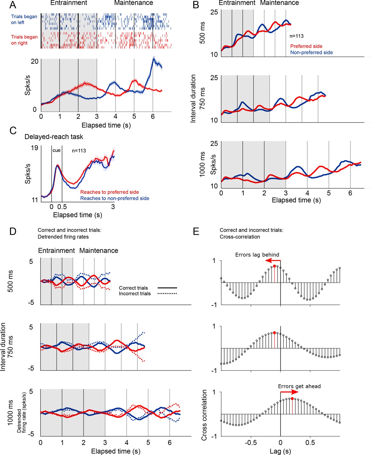
Firing patterns of SMA neurons.
(A) Rasterplot and firing rate of a representative SMA neuron during the metronome task. This neuron fires more when the stimulus is shown (entrainment), or is estimated to be (maintenance), on the right side of the screen. The panel below shows the mean firing rates for two kind of trials. (B) Mean firing rate for the 113 recorded neurons show the oscillatory nature of the activity that indicates whether the stimulus is within its preferred location, or on the opposite side. Also note the increase in mean firing rates correlated with total elapsed time. (C) Mean firing rates of the 113 neurons recorded during the delayed-reach control task. Since the delay period had variable times (randomly selected from an exponential distribution), as time progresses fewer trial contribute to the mean (Materials and methods). (D) Detrended mean firing rates and its comparison with activity on error trials. Note how the detrending allows for a better appreciation of the oscillatory patterns of correct and incorrect trials. (E) To determine if errors were lagging behind or getting ahead of the correct tempo we calculated the cross-correlation between correct and incorrect trials for the three tempos. The upper panel, corresponding the 500 ms tempo, shows a negative lag, meaning that errors were oscillating at a slower pace as compared to correct to correct trials. The opposite effect is demonstrated on the lowest panel, corresponding to the 1000 ms tempo.
Figure 7—figure supplement 1
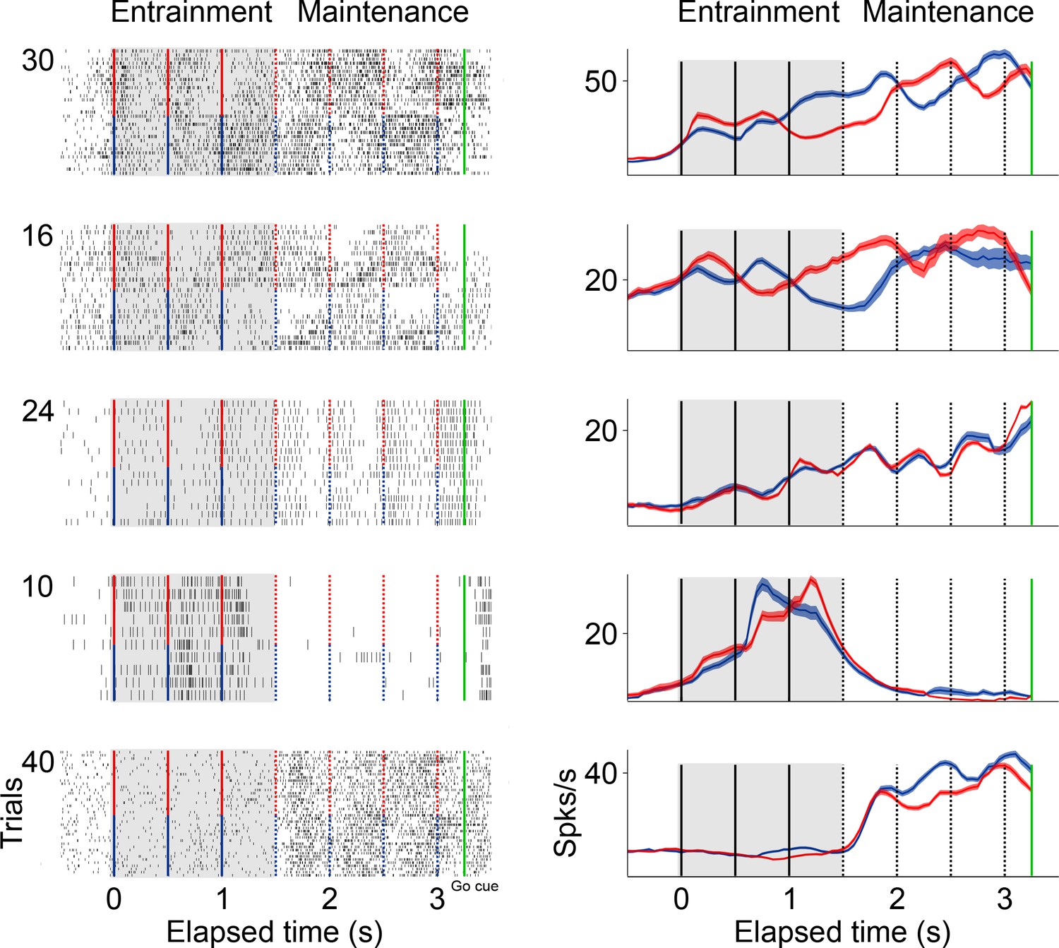
Firing patterns of single neurons during the visual metronome task.
The panels on the left column show the raster plots of five example neurons during entrainment and maintenance intervals of the task. Green lines indicate the go-cue at the last maintenance interval. Red markers indicate intervals in trials where the stimulus initiated on the right, and blue markers when the stimulus initiated on the left. Panels on the right show the mean firing rate of each neuron. Firing patterns in SMA are diverse. The first two neurons (top to bottom) have preference for one side of the screen. The third neuron oscillates in sync with the stimulus tempo but shows no side preference. The fourth neuron is mostly active during the last two entrainment intervals. The fifth neuron is mostly active during the maintenance intervals.
-
Figure 7—figure supplement 1—source data 1
Source data for the STA figures.
- https://doi.org/10.7554/eLife.38983.022
Figure 8

Relationship between spikes and LFP during the visual metronome task.
(A) The three panels on the left show the spike-triggered average (STA) of the LFP signal surrounding each individual spike of an example neuron (−100 to 100 ms window centered at each spike time). The STA of three epochs is shown; baseline (cyan), entrainment (blue), and maintenance (red). Panels on the right show the power spectrum of the STA on each epoch. (B) Average STA power across neurons. Colors denote trial epochs. Note the salient power of the STA around 30 Hz (colored areas show s.e.m. across neurons; n = 113). (C) Average STA power for periods of stimulus switch and non-switch (windows of half the interval length, centered at times of switch or at the middle of each interval; colored areas show s.e. across neurons). Dotted lines and gray areas show the STA power obtained by jittering the spikes ± 15 ms. (D) Coherence between the LFPs in simultaneously recorded electrodes, as a function of distance between them. The negative slope suggests that the recorded LFPs are generated by neuronal circuits in the vicinity of the recording electrodes.
-
Figure 8—source data 1
Source data for the STA figures.
- https://doi.org/10.7554/eLife.38983.024
Additional files
-
Transparent reporting form
- https://doi.org/10.7554/eLife.38983.025
Download links
A two-part list of links to download the article, or parts of the article, in various formats.
Downloads (link to download the article as PDF)
Open citations (links to open the citations from this article in various online reference manager services)
Cite this article (links to download the citations from this article in formats compatible with various reference manager tools)
Entrainment and maintenance of an internal metronome in supplementary motor area
eLife 7:e38983.
https://doi.org/10.7554/eLife.38983


