S-cone photoreceptors in the primate retina are functionally distinct from L and M cones
- University of Washington, United States
- Howard Hughes Medical Institute, University of Washington, United States
- Google Inc., United States
- University of Wisconsin School of Medicine and Public Health, United States
Figures
Figure 1
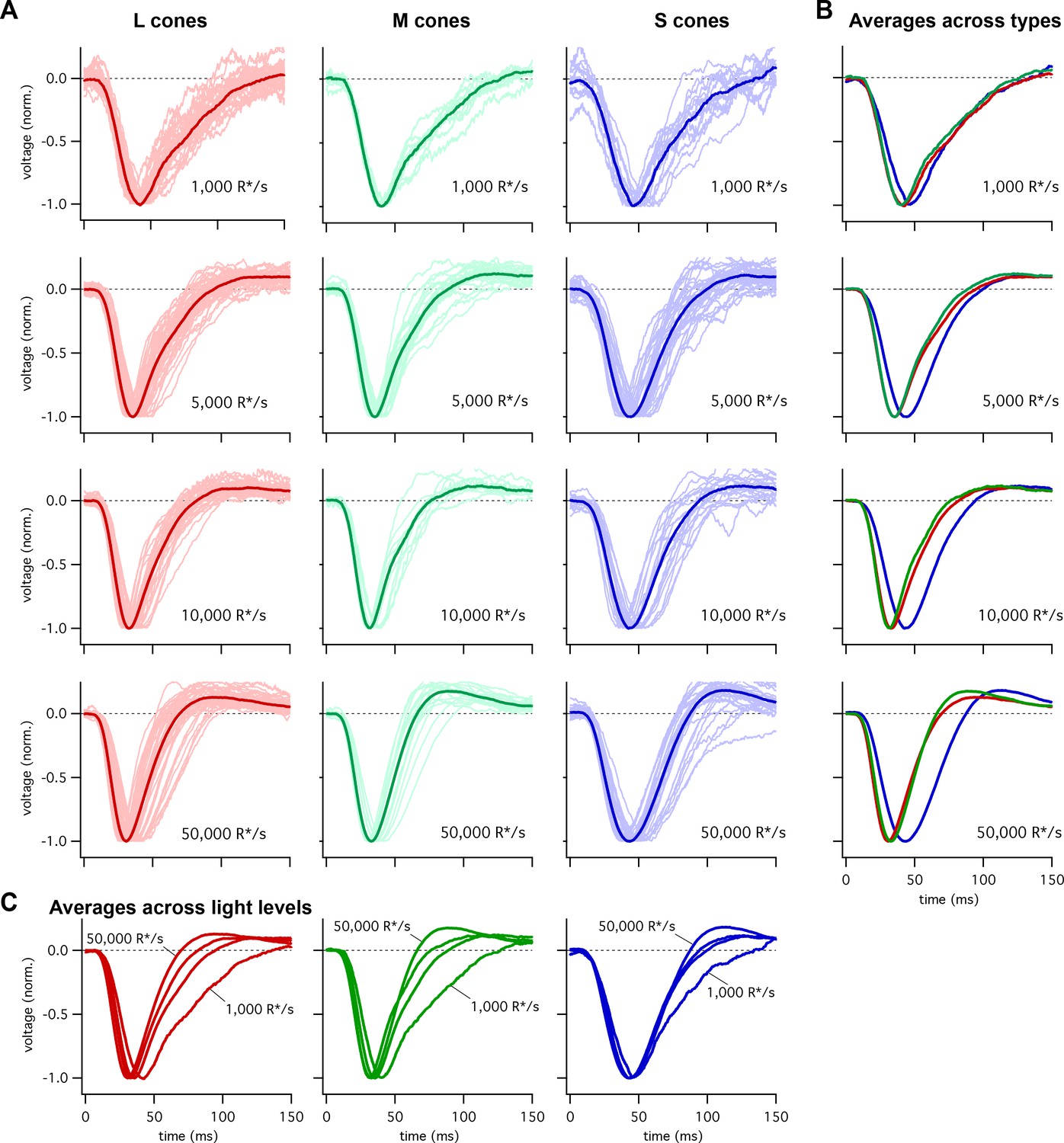
Collected flash responses from each recorded peripheral cone across backgrounds.
(A) Thin traces show voltage responses of individual cones to a 10 ms flash across several background-light levels. Traces are averages of 5–10 trials, and have been normalized in each cell. Thick traces show averages across cells. Data in this figure is collected from >10 retinas. (B) Superimposed average responses of each cone type, organized by background-light level. (C) Superimposed average responses across backgrounds, organized by cone type.
Figure 2 with 2 supplements
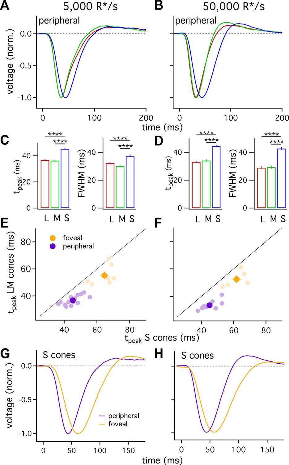
S cones are slower than L and M cones across retinal eccentricities.
(A) Average normalized voltage responses of L, M and S cones on a background of 5000 R*/s. These averages, unlike those in Figure 1, include only cells from scatter plots in E. Data in this figure is collected from >10 peripheral retinae and >= 5 foveae. (B) As in A for data collected on a background of 50,000 R*/s. Only cells from scatter plots in F are included. (C) Times to peak (left) and full-width-at-half-maximum (FWHM, right) across cone types at a background of 5000 R*/s. The mean ± sem times to peak were 36.7 ± 0.6 ms for L cones (n = 49), 36.3 ± 0.6 ms for M cones (n = 26), and 45.3 ± 0.9 ms for S cones (n = 36). p-Values from unpaired t-test. For the same cones, mean ±sem of the FWHM was 37.5 ± 1 ms for S cones, 30.2 ± 0.8 ms for M cones and 32.2 ± 0.9 ms for L cones. **** denotes p<0.0001. (D) Times to peak and FWHM as in C at 50,000 R*/s. The mean ± sem times to peak were 33.1 ± 0.7 ms for L cones (n = 42), 34.1 ± 0.9 ms for M cones (n = 17), and 44.5 ± 0.9 ms for S cones (n = 28). For the same cones, mean ±sem of the FWHM was 42.7 ± 1.1 ms for S cones, 29.4 ± 1.1 ms for M cones and 29.0 ± 1.0 ms for L cones). (E) Average time to peak of S cones compared to average time to peak of pooled L and M cones in peripheral (purple) and foveal (gold) retina on a background of 5000 R*/s. Each lightly shaded point represents the average time to peak from a single piece of retina (15 peripheral and seven foveal pieces; peripheral cells are those from A and C; foveal data comprises 29 S cones, 24 M cones and 25 L cones). Dark points with error bars represent the mean ±sem across all pieces at a given eccentricity. S cones are significantly slower than their LM counterparts in peripheral (p<10−6, paired t-test) and foveal (p<0.05, paired t-test) retina. (F) As in E, for data collected on a background of 50,000 R*/s. Peripheral (p<10−6, paired t-test) and foveal (p<0.05, paired t-test) S cones were significantly slower than their LM counterparts (11 peripheral pieces, five foveas; peripheral cells are those from B and D; foveal data comprises 21 S cones, 8 M cones, and 12 L cones). (G) Average S-cone flash responses from peripheral and foveal retina on a background of 5,000 R*/s. Times to peak of 63.5 ± 1.8 ms for 29 foveal S cones and 45.3 ± 0.9 ms for 36 peripheral S cones. (H) As in (G) on a background of 50,000 R*/s. Times to peak of 59.1 ± 2.1 ms for 21 foveal S cones and 44.5 ± 0.9 ms for 28 peripheral S cones.
Figure 2—figure supplement 1
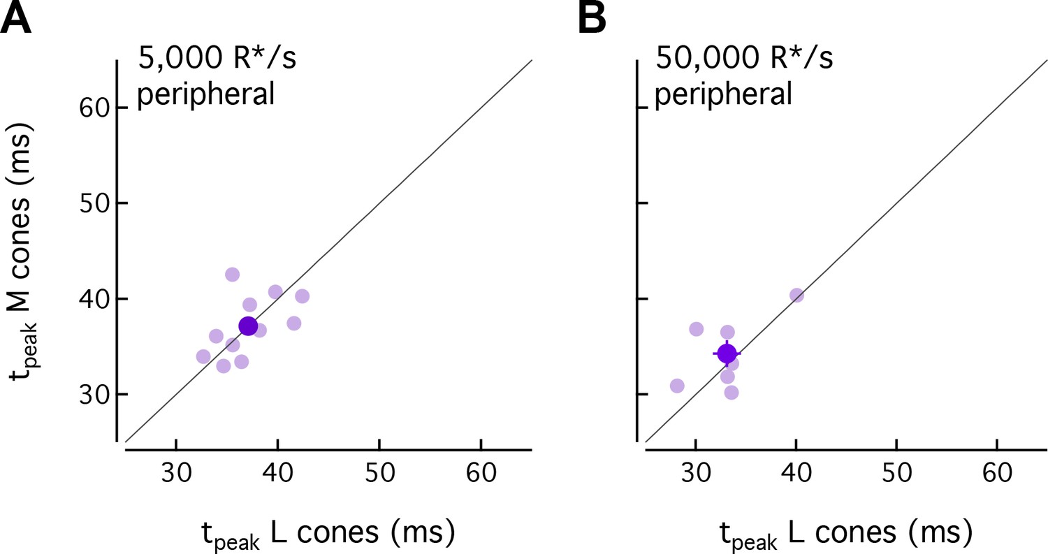
Kinetics of L- and M-cone flash responses are similar.
(A) Average time to peak of L cones (n = 29) compared to average time to peak of M cones (n = 26) in peripheral retina on a background of 5000 R*/s. Each light purple point represents the average times to peak from a single piece of retina. The dark purple point with error bars represents mean ±sem across all pieces. (B) As in panel A for data collected on a background of 50,000 R*/s, 17 M cones and 42 L cones.
Figure 2—figure supplement 2
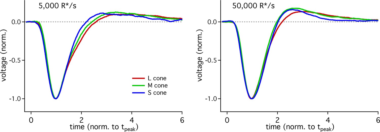
S and LM cones have similar response shapes Left and right panels superimpose average responses from each cone type with the peak absolute amplitude and the time to peak normalized to one.
With this normalization, the responses of different cone types are quite similar. Hence, the differences in kinetics illustrated in Figures 1 and 2 are not due to a preferential slowing of either the rising or falling phase of the response (see Discussion).
Figure 3
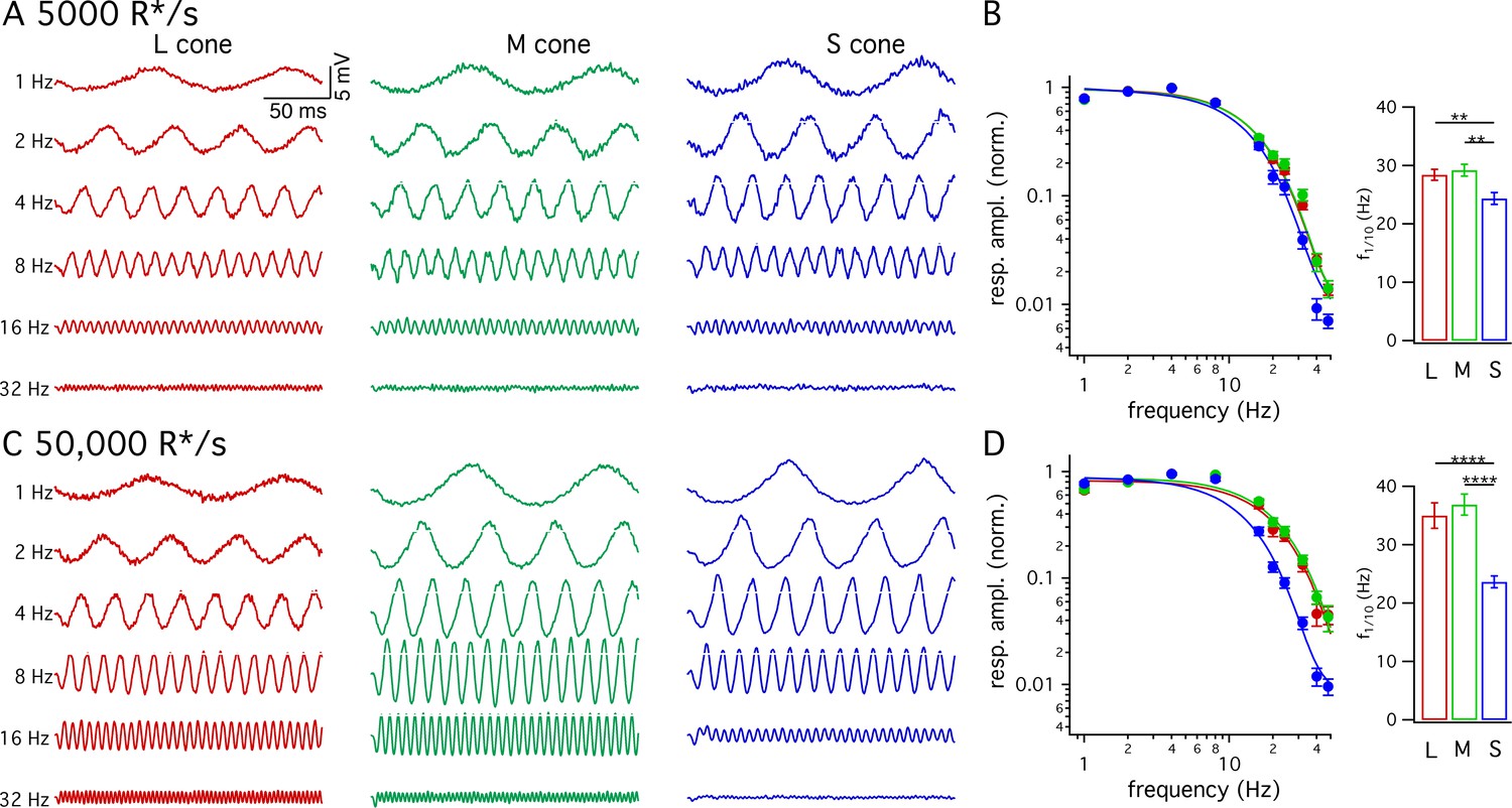
Frequency tuning differs for S and LM cones.
(A) Voltage responses to sinusoidal stimuli across a range of frequencies from example L, M and S cones. Mean light level 5000 R*/s. Stimulus contrast increased with increasing temporal frequency to avoid saturating responses at low frequencies. Data in this figure is collected from >10 retinas. (B) Frequency tuning curves across cone types. Points with error bars are mean ± sem temporal frequency sensitivities of L, M and S cones on a background of 5000 R*/s. Values are the normalized response amplitudes across frequencies. Curves show best fit of power spectrum of Equation 1 to the population data. Right panel shows mean ±sem frequencies at which response amplitudes decreased to 10% of their maximum value, which were 28.4 ± 0.9 Hz in L cones (n = 26), 29.2 ± 1.0 Hz in M cones (n = 17), and 24.4 ± 1.0 Hz in S cones (n = 15). P values from unpaired t-test; ** denotes p<0.01 (C) Responses from the same cones and frequencies as A at 50,000 R*/s. (D) As in B for data collected on a background of 50,000 R*/s. Mean ± sem temporal frequencies for 10% maximum gain were 35.0 ± 2.2 Hz in L cones (n = 17), 36.9 ± 1.8 Hz in M cones (n = 21), and 23.6 ± 1.0 Hz in S cones (n = 16). **** denotes p<0.0001.
Figure 4
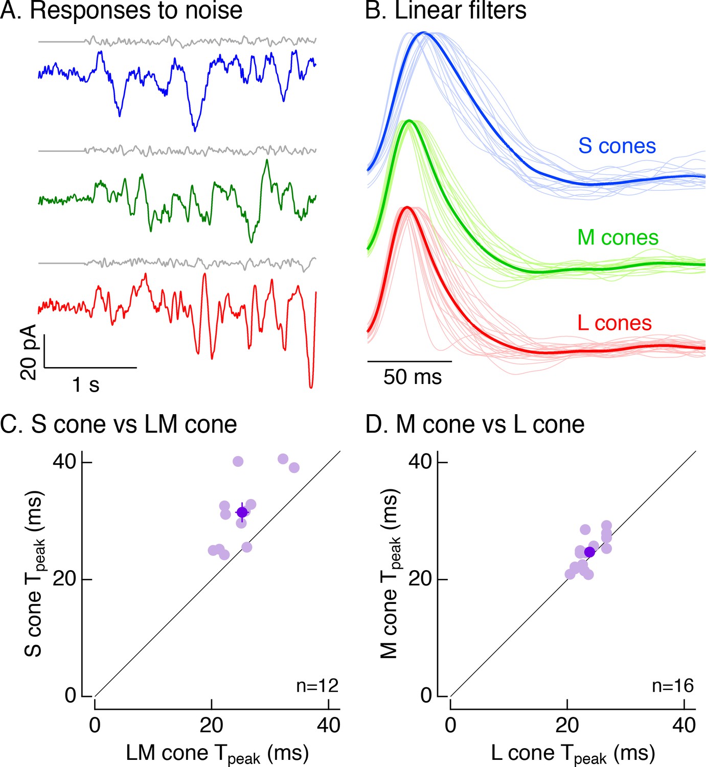
Cone photocurrents differ in kinetics.
(A) Example current responses of a voltage-clamped S (top), M (middle) and L (bottom) cone to a short section of Gaussian-modulated light input (gray). The background to which modulation was added produced on average 2500 R*/s in each case. Responses were low-pass filtered digitally with a 100 Hz cutoff. Data in this figure is collected from at least 8 retinas. (B) Normalized linear filters of L, M and S cones on a background of 2500 R*/s. Filters were calculated to be those that optimally map Gaussian-noise stimuli to measured cone responses. Thick traces show average filters, thin traces filters from individual cones (17 S cones, 17 M cones, 24 L cones from nine retinas). (C) Comparison of times to peak of S-cone versus LM-cone linear filters. Each open circle represents the times to peak of filters from an S cone and an L or M cone from the same piece of retina (12 S cones from eight retinas). Closed circle plots mean ±sem. S-cone times to peak were significantly shorter than in LM cones (31.5 ± 2 ms for S cones vs 25.2 ± 1.2 ms for paired LM cones, p<0.005, paired t-test). There are fewer cones here than in B because not every S cone could be paired with an LM cone. (D) Comparison of times to peak of M-cone versus L-cone linear filters as in C. L-and M-cone times to peak were not significantly different (p>0.05, paired t-test; 16 M cones across nine retinas, 24.7 ± 0.7 ms for M cones vs 23.8 ± 0.5 ms for paired L cones).
Figure 5 with 1 supplement
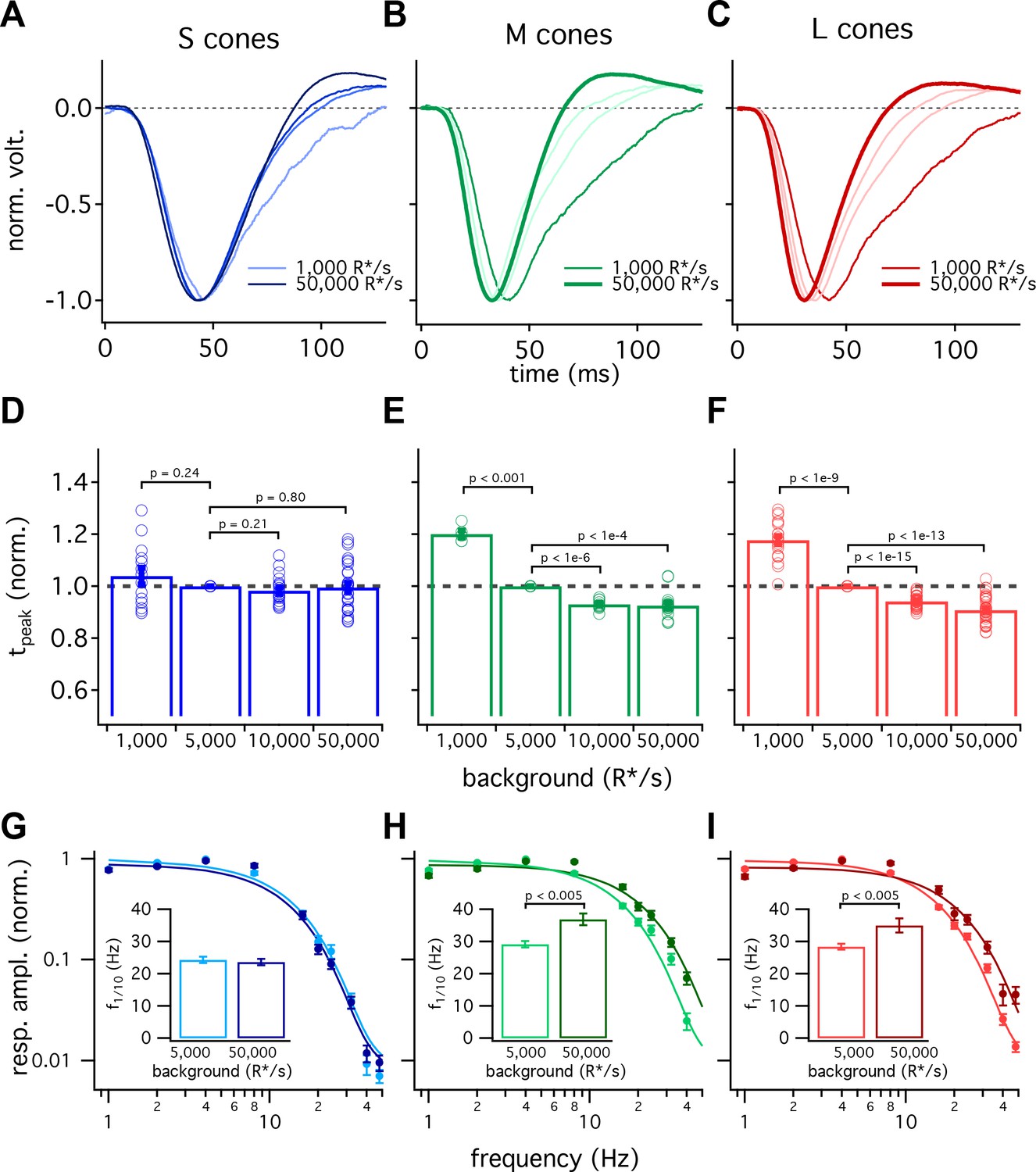
S-cone kinetics change minimally across background light levels.
(A–C) Average normalized voltage responses of S (A), M (B), and L (C) cones on backgrounds of 1000 R*/s (thin line) and 50,000 R*/s (thick line); data replotted from Figure 1C. Lighter lines show responses at intermediate light levels of 5000 R*/s and 10,000 R*/s. Total of 36 S cones, 26 M cones and 49 L cones. Data in this figure is collected from >10 retinas. (D–F) Mean ± sem relative times to peak across backgrounds in S (D), M (E), and L (F) cones. In each cell, the time to peak at each background was normalized by the time to peak at 5000 R*/s in that cell. p-Values from one-sample t-test. (G–I) Frequency-tuning curves at 5000 R*/s and 50,000 R*/s in S (G), M (H), and L (I) cones. Points with error bars are mean ± sem normalized response amplitudes across frequencies. Curves show fit of power spectrum of Equation 1 to population data. Inset shows mean ± sem frequencies at which response amplitudes decreased to 10% of their maximum value at either background. At 5000 and 50,000 R*/s, these frequencies were 24.4 ± 1.0 Hz (n = 15) and 23.6 ± 1.0 Hz (n = 16) in S cones, 29.2 ± 1.0 Hz (n = 17) and 36.9 ± 1.8 Hz (n = 21) in M cones, and 28.4 ± 0.9 Hz (n = 26) and 35.0 ± 2.2 Hz (n = 17) in L cones. p-Values from unpaired t-test.
Figure 5—figure supplement 1
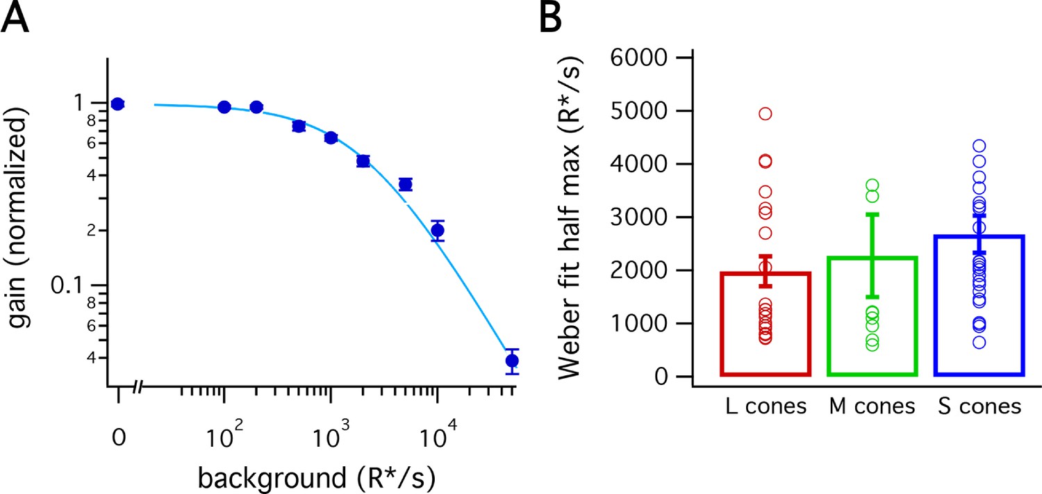
Response amplitude adaptation across cone types.
(A) Response amplitude adaptation in S cones. Points with error bars represent mean ±sem normalized gains across backgrounds. Prior to averaging, values from each cell were fit to Equation 2.4 and scaled such that the gain of the fit on a background of 0 R*/s was 1. Solid line shows fit of Equation 2.4 to population data, demonstrating that S cone adaptation can be described by this equation. (B) Half-maximum backgrounds from Weber curve (Equation 4) fits to amplitude adaptation data in each cone type (25 S cones, 9 M cones, 22 L cones). Error bars represent sem. Weber fit half-maximum values are not significantly different across cone types (p=0.43, one-way ANOVA).
Figure 6
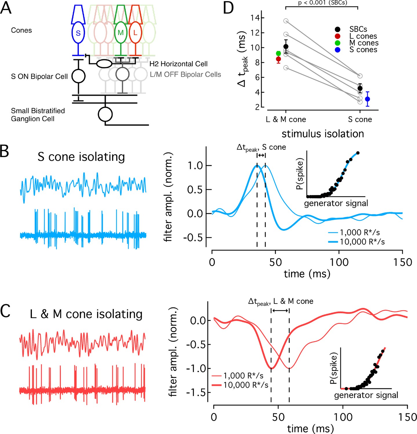
Differences in cone adaptation affect retinal ganglion cell responses.
(A) Previously described circuitry upstream of SBCs. S-ON signals travel from S cones through S-ON Bipolar Cells to SBCs. L/M-OFF signals travel from L and M cones through H2 horizontal cells to S-cone terminals, where they are transmitted to SBCs via S-ON Bipolar cells. Alternatively, L- and M-cone signals may be carried to SBCs directly via an L/M-OFF Bipolar cell. Data in this figure is collected from two retinas. (B) Example response of SBC to S-cone isolating Gaussian-noise stimulus (left). Example Linear-nonlinear (LN) model derived from SBC responses to Gaussian-noise stimuli (right). Normalized linear filters shown for backgrounds of 1000 and 10,000 R*/s. Time-to-peak shifts between 1000 R*/s and 10,000 R*s were taken to be the difference in the times to peak of the linear filters at each background. Inset shows nonlinearity mapping from generator signal to spiking probability. (C) Example response and LN Model as in (C), but for L/M-OFF response. (D) Comparison of time-to-peak shifts in S-ON and L/M-OFF SBC responses. Mean ± sem shifts were 10.2 ± 0.9 ms for L/M-OFF responses and 4.5 ± 0.6 ms for S-ON responses (n = 6). Shifts in each cone type between 1,000 and 10,000 R*/s are shown for comparison. Shifts were 3.1 ± 1.0 ms in S cones (n = 14), 9.2 ± 0.3 ms in M cones (n = 7), and 8.49 ± 0.6 ms in L cones (n = 22). P value from paired t-test.
Figure 7 with 1 supplement
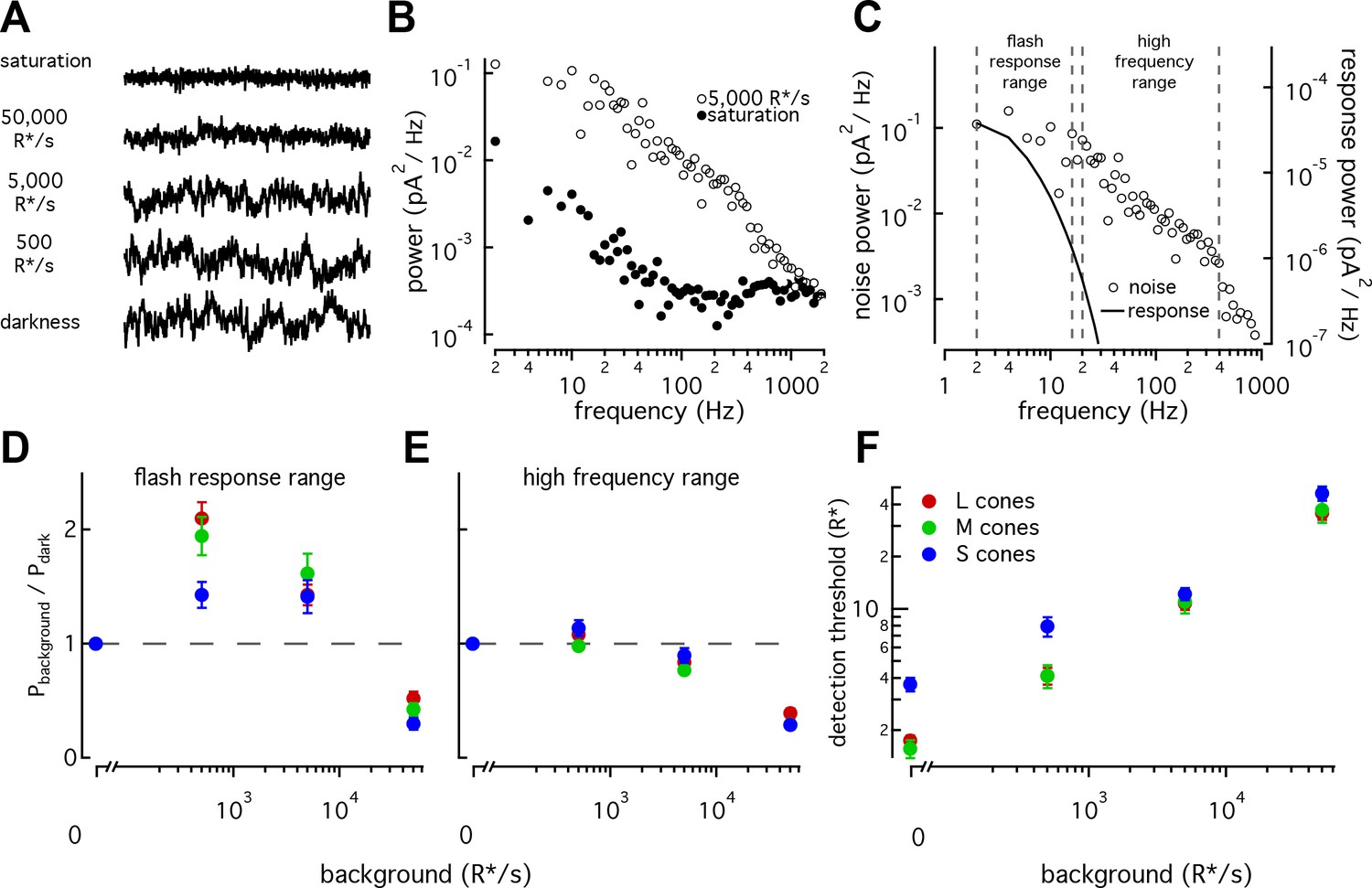
S cones have lower signal-to-noise ratios under dim-lighting conditions.
(A) Example current recordings from an S cone on backgrounds of 0, 500, 5000, and 50,000 R*/s and in saturating light. Data in this figure is collected from >10 retinas. (B) Example power spectra of noise at 5000 R*/s (open circles) and in saturating light (closed circles) from an S cone. Spectrum at 5000 R*/s includes contributions from cellular as well as instrumental noise. (C) Example isolated cellular noise spectrum (left axis, open circles) and flash response spectrum (right axis, solid line), both on a background of 5000 R*/s. Dashed vertical lines identify bounds for flash-response and high-frequency ranges used in (D–F) (Flash-response range: 2–16 Hz; high-frequency range: 20–394 Hz). (D) Noise power in flash-response range in S (n = 14), M (n = 18), and L (n = 29) cones. Values show mean ± sem powers across backgrounds normalized by the power in darkness. Dashed horizontal line shows noise power in darkness. The change in S-cone noise at 500 R*/s was significantly lower than that in L and M cones (S vs M, p<0.05; S vs L, p<0.001; unpaired t-test). (E) As in (D) but for noise in high-frequency range. (F) Detection thresholds across backgrounds in S (n = 9), M (n = 9) and L (n = 15) cones. Plotted values show mean ±sem. In darkness, mean ± sem threshold is 3.67 ± 0.33 R* in S cones, 1.57 ± 0.18 R* in M cones, and 1.75 ± 0.12 R* in L cones. At 500 R*/s it is 7.95 ± 1.02 R* in S cones, 4.13 ± 0.63 R* in M cones, and 4.12 ± 0.46 R* in L cones.
Figure 7—figure supplement 1
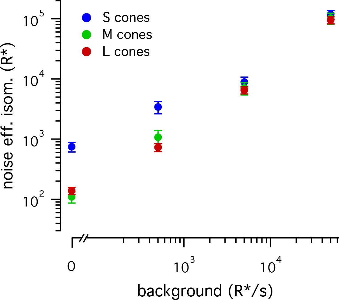
Noise-effective isomerizations across cone types Effective noise-isomerization levels across backgrounds.
Values were computed as number of isomerizations necessary to produce an equivalent power to the noise in the range of 2 to 16 Hz. Points represent mean ±sem. For S cones (n = 9), values were 737 ± 136 R* in darkness, 3422 ± 780 R* at 500 R*/s, 8914 ± 1848 R* at 5000 R*/s, and 117,419 ± 19,785 R* at 50,000 R*/s. For M cones (n = 9), values were 110 ± 23 R* in darkness, 3422 ± 780 R* at 500 R*/s, 7050 ± 1624 R* at 5000 R*/s, and 102,721 ± 21,195 R* at 50,000 R*/s. For L cones (n = 15), values were 139 ± 19 R* in darkness, 731 ± 110 R* at 500 R*/s, 6522 ± 879 R* at 5000 R*/s, and 95,295 ± 12,725 R* at 50,000 R*/s.
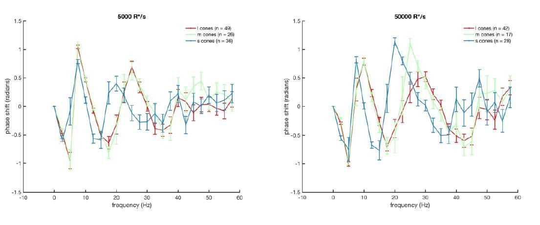
Author response image 1

Author response image 2
Tables
Key resources table
| Reagent type (species or resource | Designation | Source or reference | Identifiers | Additional information |
|---|---|---|---|---|
| Antibody | anti-OPN1SW (Mouse monoclonal) | Santa CruzBiotechnology | Cat#: sc14363 | (1:50) |
| Antibody | anti-goat IgG (H + L) HiLyte Fluor 750 | AnaSpec | (1:100) Secondary antibody | |
| Biological Samples | Macaque retina | Washington Regional Primate Research Centre | N/A | Macaca fascicularis, Macaca nemestrina, and Macaca mulatta of both sexes, aged 2 through 20years |
| Chemical compound, drug | Ames | Sigma | 1420 | |
| Chemical compound, drug | DNase1 | Sigma | 11284932001 | |
| Software, Algorithms | IGOR Pro | WaveMetrics | https://www.wavemetrics.com/ | |
| Software, Algorithms | MATLAB | Mathworks | https://ch.mathworks.com/products/matlab | |
| Software, Algorithms | Symphony | Symphony-DAS | http://symphony-das.github.io/ |
Additional files
-
Transparent reporting form
- https://doi.org/10.7554/eLife.39166.013
Download links
A two-part list of links to download the article, or parts of the article, in various formats.
Downloads (link to download the article as PDF)
Open citations (links to open the citations from this article in various online reference manager services)
Cite this article (links to download the citations from this article in formats compatible with various reference manager tools)
S-cone photoreceptors in the primate retina are functionally distinct from L and M cones
eLife 8:e39166.
https://doi.org/10.7554/eLife.39166


