Adaptation of olfactory receptor abundances for efficient coding
- Flatiron Institute, United States
- City University of New York, United States
- University of Pennsylvania, United States
- École Normale Supérieure and CNRS UMR 8550, PSL Research, UPMC Sorbonne Université, France
Figures
Figure 1
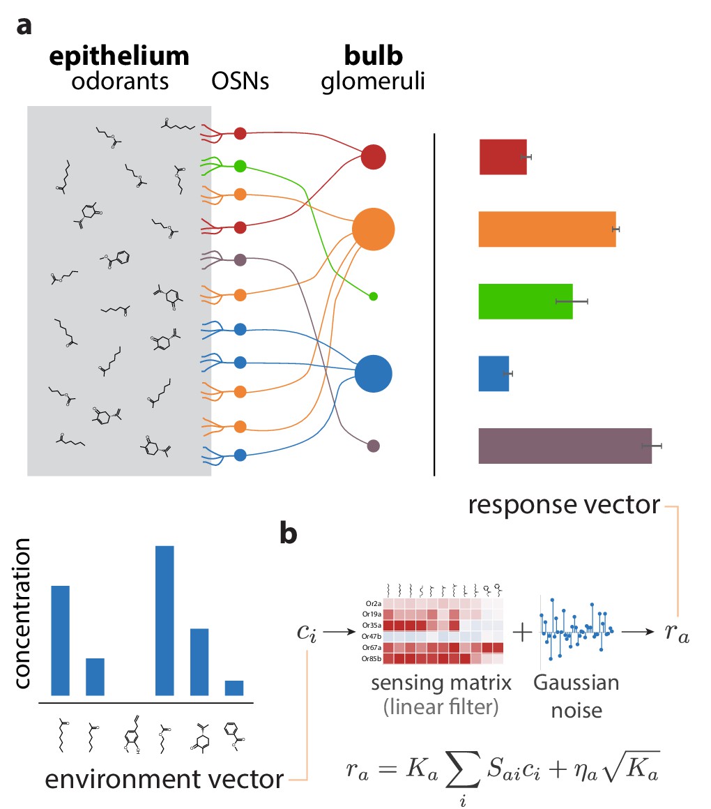
Sketch of the olfactory periphery as described in our model.
(a) Sketch of olfactory anatomy in vertebrates. The architecture is similar in insects, with the OSNs and the glomeruli located in the antennae and antennal lobes, respectively. Different receptor types are represented by different colors in the diagram. Glomerular responses (bar plot on top right) result from mixtures of odorants in the environment (bar plot on bottom left). The response noise, shown by black error bars, depends on the number of receptor neurons of each type, illustrated in the figure by the size of the corresponding glomerulus. Glomeruli receiving input from a small number of OSNs have higher variability due to receptor noise (e.g., OSN, glomerulus, and activity bar in green), while those receiving input from many OSNs have smaller variability. Response magnitudes depend also on the odorants present in the medium and the affinity profile of the receptors. (b) We approximate glomerular responses using a linear model based on a ‘sensing matrix’ , perturbed by Gaussian noise . are the numbers of OSNs of each type.
Figure 2
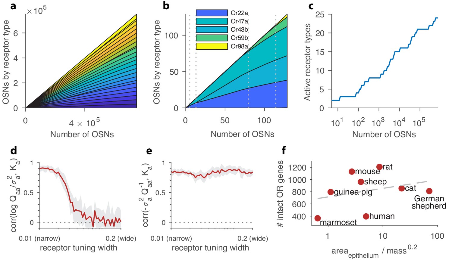
Structure of a well-adapted receptor distribution.
In panels (a–c) the receptor sensing matrix is based on Drosophila (Hallem and Carlson, 2006) and includes 24 receptors responding to 110 odorants. In panels (d–e), the total number of OSNs is fixed at 4000. In all panels, environmental odor statistics follow a random correlation matrix (see Appendix 4). Qualitative aspects are robust to variations in these choices (see Appendix 1). (a) Large OSN populations should have high receptor diversity (types represented by strips of different colors), and should use receptor types uniformly. (b) Small OSN populations should express fewer receptor types, and should use receptors non-uniformly. (c) New receptor types are expressed in a series of step transitions as the total number of neurons increases. Here, the odor environments and the receptor affinities are held fixed as the OSN population size is increased. (d) Correlation between the abundance of a given receptor type, , and the logarithm of its signal-to-noise ratio in olfactory scenes, , shown here as a function of the tuning of the receptors. For every position along the -axis, sensing matrices with a fixed receptor tuning width were generated from a random ensemble, where the tuning width indicates what fraction of all odorants elicit a strong response for the receptors (see Appendix 1). When each receptor responds strongly to only a small number of odorants, response variance is a good predictor of abundance, while this is no longer true for wide tuning. (e) Receptor abundances correlate well with the diagonal elements of the inverse overlap matrix normalized by the noise variances, , for all tuning widths. In panels (d–e), the red line is the mean obtained from 24 simulations, each performed using a different sensing matrix, and the light gray area shows the interval between the 20th and 80th percentiles of results. (f) Number of intact olfactory receptor (OR) genes found in different species of mammals as a function of the area of the olfactory epithelium normalized to account for allometric scaling of neuron density ((Herculano-Houzel et al., 2015); see main text). We use this as a proxy for the number of neurons in the olfactory epithelium. Dashed line is a least-squares fit. Number of intact OR genes from (Niimura et al., 2014), olfactory surface area data from (Moulton, 1967; Pihlström et al., 2005; Gross et al., 1982; Smith et al., 2014), and weight data from (Rousseeuw and Leroy, 1987; FCI, 2018; Gross et al., 1982; Smith et al., 2014).
Figure 3
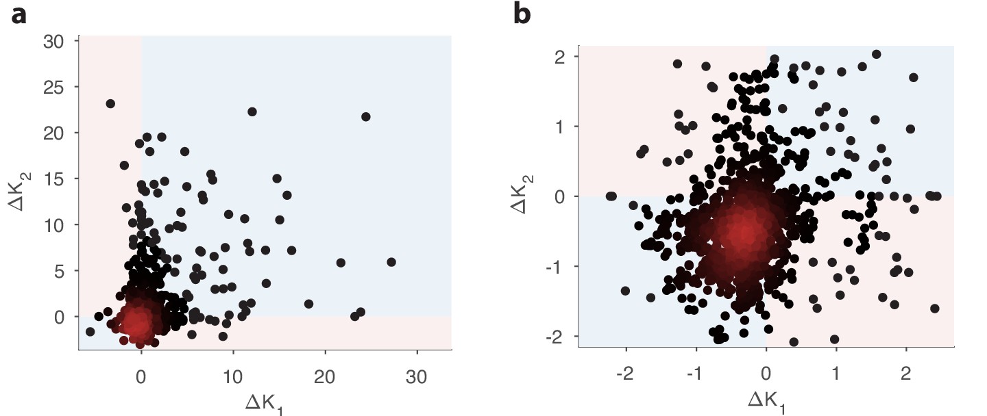
Comparison of changes in receptor abundances when the same perturbation is applied to two different environments.
One hundred different pairs of environments were generated, with each environment defined by a random odor covariance matrix (procedure in Appendix 4, parameter ). In each pair of environments (), the variance of a randomly chosen odorant was increased (details in Appendix 4) to produce perturbed environments. For each receptor, we computed the optimal abundance before and after the perturbation ( and ) and computed the differences . The background environments in each pair set the context for the adaptive change after the perturbation. We used a sensing matrix based on fly affinity data (Hallem and Carlson, 2006) (24 receptors, 110 odors) and set the total OSN number to . Panel (b) zooms in on the central part of panel (a). In light blue regions, the sign of the abundance change is the same in the two contexts; light pink regions indicate opposite sign changes in the two contexts. In both figures, dark red indicates high-density regions where there are many overlapping data points.
Figure 4

Effect of changing environment on the optimal receptor distribution.
(a) An example of an environment with a random odor covariance matrix with a tunable amount of cross-correlation (details in Appendix 4). The variances are drawn from a lognormal distribution. (b) Close-ups showing some differences between the two environments used to generate results in (c and d). The two covariance matrices are obtained by adding a large variance to two different sets of 10 odorants (out of 110) in the matrix from (a). The altered odorants are identified by yellow crosses; their variances go above the color scale on the plots by a factor of more than 60. (c) Change in receptor distribution when going from environment 1 to environment 2, in conditions where the total number of receptor neurons is large (in this case, ), and thus the SNR is high. The blue diamonds on the left correspond to the optimal OSN fractions per receptor type in the first environment, while the orange diamonds on the right correspond to the second environment. In this high-SNR regime, the effect of the environment is small, because in both environments the optimal receptor distribution is close to uniform. (d) When the total number of neurons is small ( here) and the SNR is low, changing the environment can have a dramatic effect on optimal receptor abundances, with some receptors that are almost vanishing in one setting becoming highly abundant in the other, and vice versa.
Figure 5
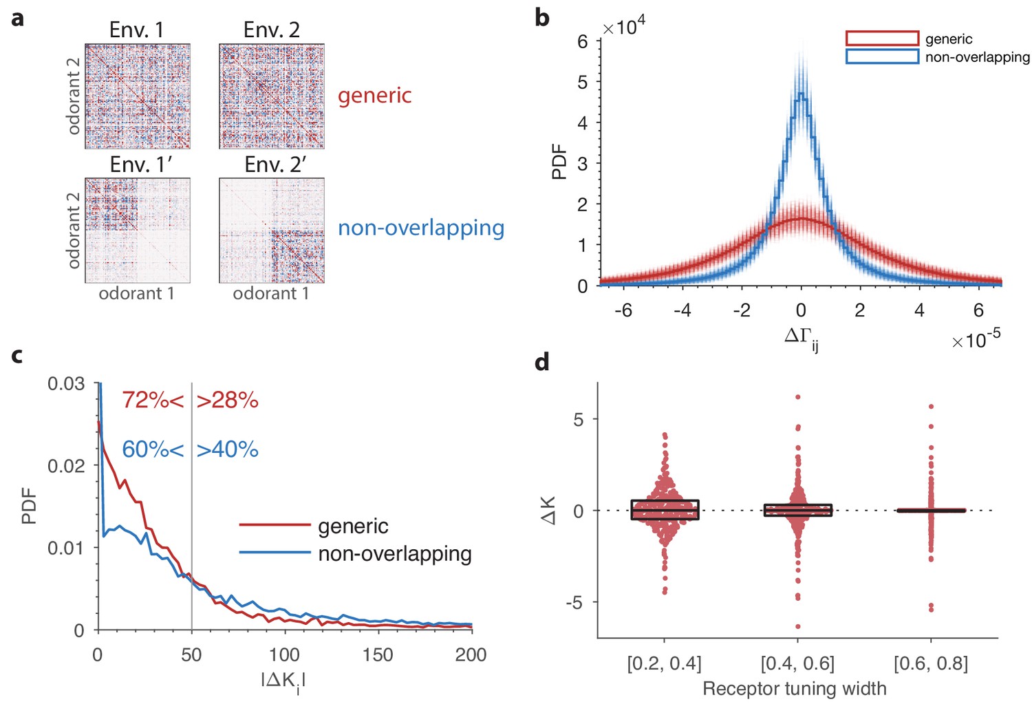
The effect of a change in environmental statistics on the optimal receptor distribution as a function of overlap in the odor content of the two environments, and the tuning properties of the olfactory receptors.
(a) Random environment covariance matrices used in our simulations (red entries reflect positive [co-]variance; blue entries reflect negative values). The environments on the top span a similar set of odors, while those on the bottom contain largely non-overlapping sets of odors. (b) The distribution of changes in the elements of the environment covariance matrices between the two environments is wider (i.e. the changes tend to be larger) in the generic case than in the non-overlapping case shown in panel (a). The histograms in solid red and blue are obtained by pooling the 500 samples of pairs of environment matrices from each group. The plot also shows, in lighter colors, the histograms for each individual pair. (c) Probability distribution functions of changes in optimal OSN abundances in the 500 samples of either generic or non-overlapping environment pairs. These are obtained using receptor affinity data from the fly (Hallem and Carlson, 2006) with a total number of neurons . The non-overlapping scenario has an increased occurrence of both large changes in the OSN abundances, and small changes (the spike near the -axis). The -axis is cropped for clarity; the maximal values for the abundance changes are around 1000 in both cases. (d) Effect of tuning width on the change in OSN abundances. Here two random environment matrices obtained as in the ‘generic’ case from panels (a–c) were kept fixed, while 50 random sensing matrices with 24 receptors and 110 odorants were generated. The tuning width for each receptor, measuring the fraction of odorants that produce a significant activation of that receptor (see Appendix 1), was chosen uniformly between 0.2 and 0.8. The receptors from all the 50 trials were pooled together, sorted by their tuning width, and split into three tuning bins. Each dot represents a particular receptor in the simulations, with the vertical position indicating the amount of change in abundance . The horizontal locations of the dots were randomly chosen to avoid too many overlaps; the horizontal jitter added to each point was chosen to be proportional to the probability of the observed change within its bin. This probability was determined by a kernel density estimate. The boxes show the median and interquartile range for each bin. The abundances that do not change at all () are typically ones that are predicted to have zero abundance in both environments, .
Figure 6
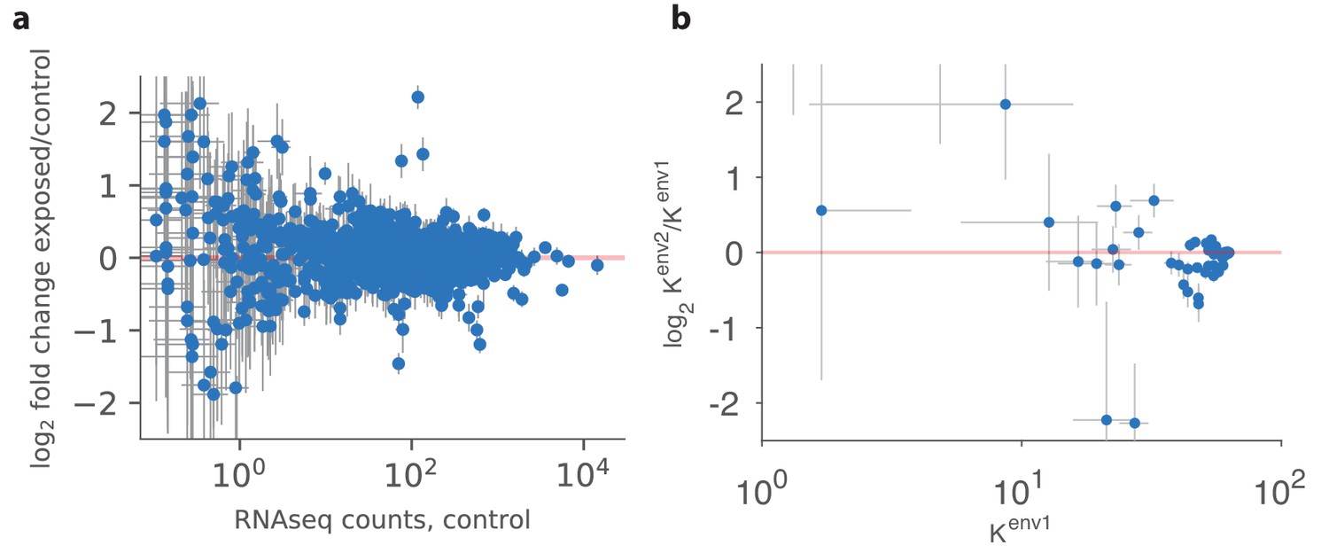
Qualitative comparison between experiment and theory.
(a) Panel reproduced from raw data in Ibarra-Soria et al. (2017), showing the log-ratio between receptor abundances in the mouse epithelium in the test environment (where four odorants were added to the water supply) and those in the control environment, plotted against values in control conditions (on a log scale). The error bars show standard deviation across six individuals. Compared to Figure 5B in Ibarra-Soria et al. (2017), this plot does not use a Bayesian estimation technique that shrinks ratios of abundances of rare receptors toward 1 (personal communication with Professor Darren Logan, June 2017). (b) A similar plot produced in our model using mouse and human receptor response curves (Saito et al., 2009). The error bars show the range of variation found in the optimal receptor distribution when slightly perturbing the two environments (see the text). The simulation includes 59 receptor types for which response curves were measured (Saito et al., 2009), compared to 1115 receptor types assayed in Ibarra-Soria et al. (2017). Our simulations used total OSNs.
Figure 7
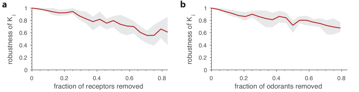
Robustness of optimal receptor distribution to subsampling of odorants and receptor types.
Robustness in the prediction is measured as the Pearson correlation between the predicted OSN numbers with complete information, and after subsampling. (a) Robustness of OSN abundances as a function of the fraction of receptors removed from the sensing matrix. Given a full sensing matrix (in this case a 24 × 110 matrix based on Drosophila data (Hallem and Carlson, 2006)), the abundances of a subset of OSN types were calculated in two ways. First, the optimization problem from Equation (7) was solved including all the OSN types and an environment with a random covariance matrix (see Figure 5). Then a second optimization problem was run in which a fraction of the OSN types were removed. The optimal neuron counts obtained using the second method were then compared (using the Pearson correlation coefficient) against the corresponding numbers from the full optimization. The shaded area in the plot shows the range between the 20th and 80th percentiles for the correlation values obtained in 10 trials, while the red curve is the mean. A new subset of receptors to be removed and a new environment covariance matrix were generated for each sample. (b) Robustness of OSN abundances as a function of the fraction of odorants removed from the environment, calculated similarly to panel a except now a certain fraction of odorants was removed from the environment covariance matrix, and from the corresponding columns of the sensing matrix.
Figure 8
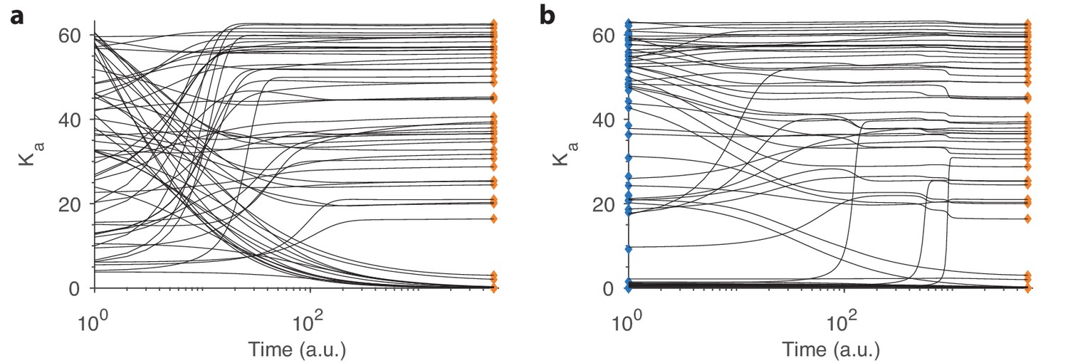
Convergence in our dynamical model.
(a) Example convergence curves in our dynamical model showing how the optimal receptor distribution (orange diamonds) is reached from a random initial distribution of receptors. Note that the time axis is logarithmic. (b) Convergence curves when starting close to the optimal distribution from one environment (blue diamonds) but optimizing for another. A small, random deviation from the optimal receptor abundance in the initial environment was added (see text).
Appendix 1—figure 1
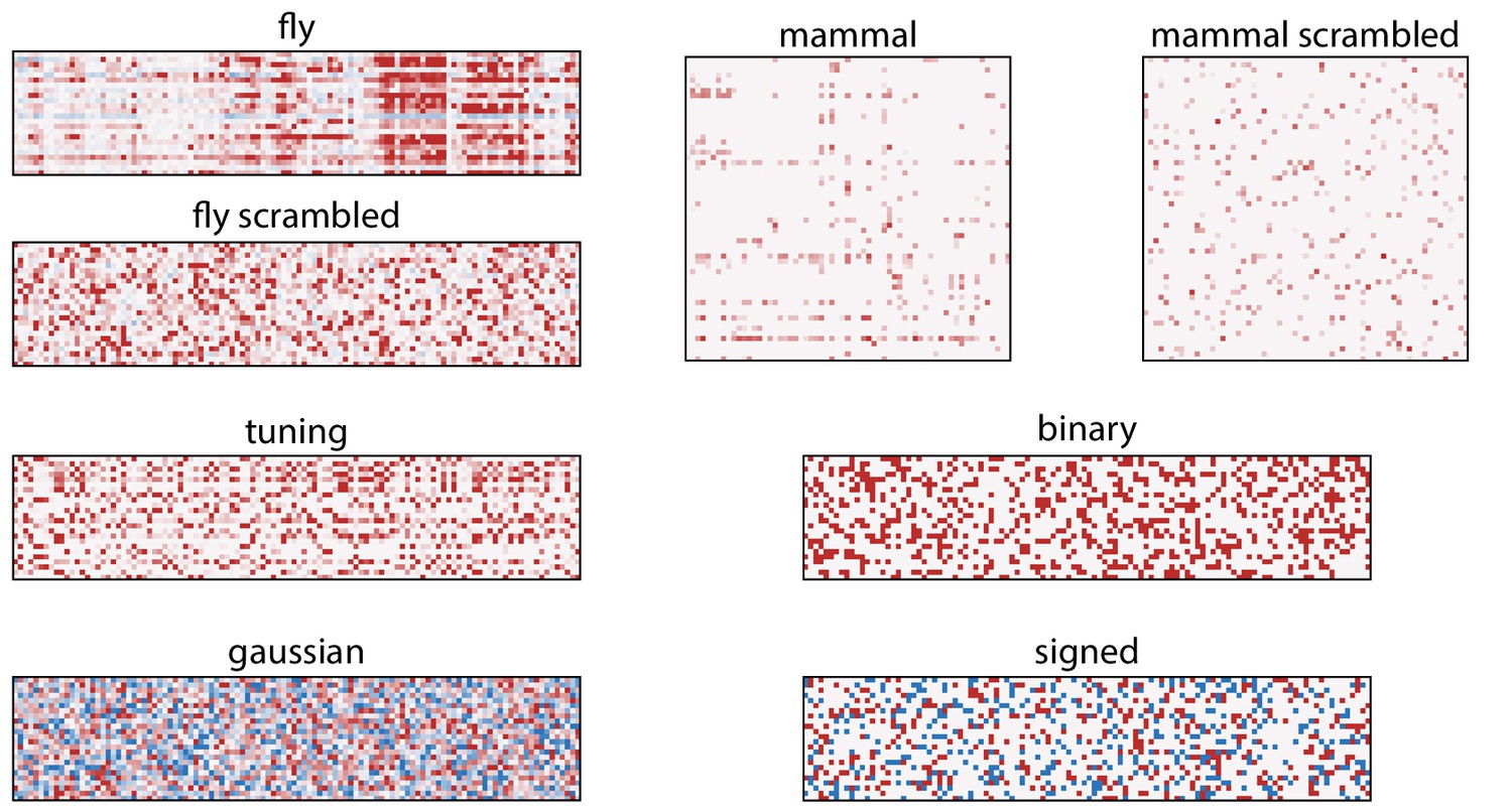
Heat maps of the types of sensing matrices used in our study.
The color scaling is arbitrary, with red representing positive values and blue negative values. ‘Fly’ and ‘mammal’ are the sensing matrices based on Drosophila receptor affinities (Hallem and Carlson, 2006), and mouse and human affinities (Saito et al., 2009), respectively. ‘Fly scrambled’ and ‘mammal scrambled’ are permutations of the ‘fly’ and ‘mammal’ matrices in which elements are arbitrarily scrambled. ‘Tuning’, ‘gaussian’, ‘binary’, and ‘signed’ are random sensing matrix generated as described in the Random sensing matrices section.
Appendix 1—figure 2
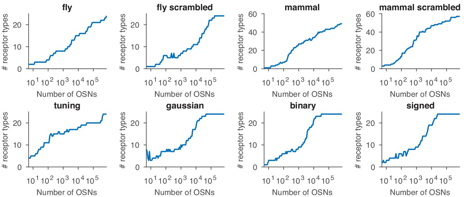
Effect of sensing matrix on the dependence between the number of receptor types expressed in the optimal distribution and the total number of OSNs.
The labels refer to the sensing matrices from Appendix 1—figure 1.
Appendix 1—figure 3
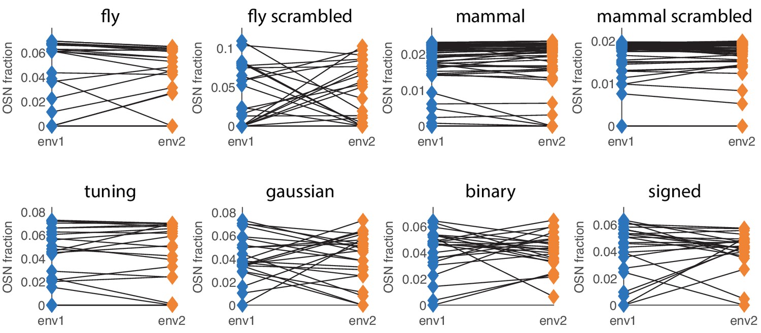
Different choices of sensing matrix lead to similar behavior of optimal receptor distribution under environment change.
The labels refer to the sensing matrices from Appendix 1—figure 1, whose scales were adjusted to ensure that the simulations are in a low SNR regime. The blue (orange) diamonds on the left (right) side of each plot represent the optimal OSN abundances in environment 1 (environment 2). The two environment covariance matrices are obtained by starting with a background randomly-generated covariance matrix (as described below) and adding a large amount of variance to two different sets of 10 odorants (out of 110 for most sensing matrices, and 63 for the ‘mouse’ and ‘mouse scrambled’ ones).
Appendix 3—figure 1
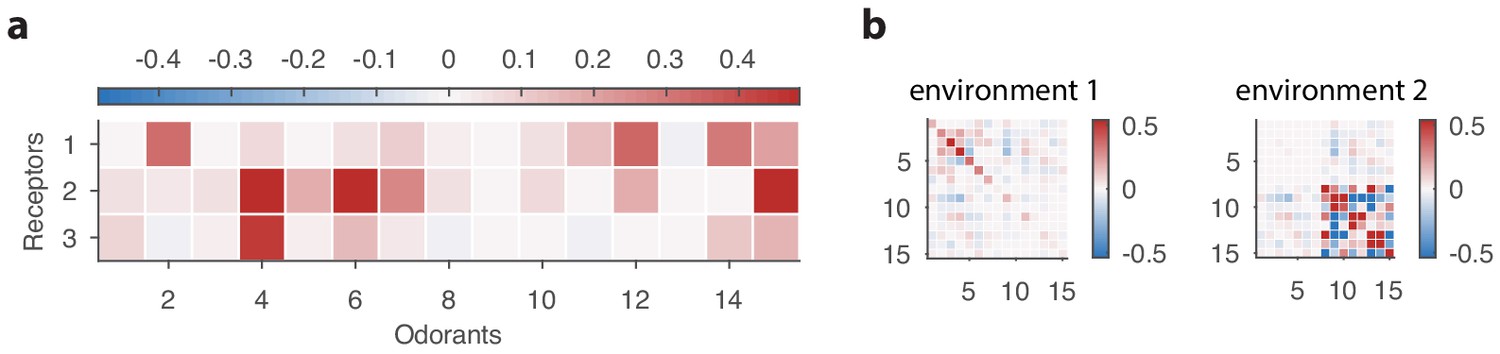
Sensing matrix and environment covariance matrices used in our toy problem involving a non-linear response function.
https://doi.org/10.7554/eLife.39279.018
Appendix 3—figure 2
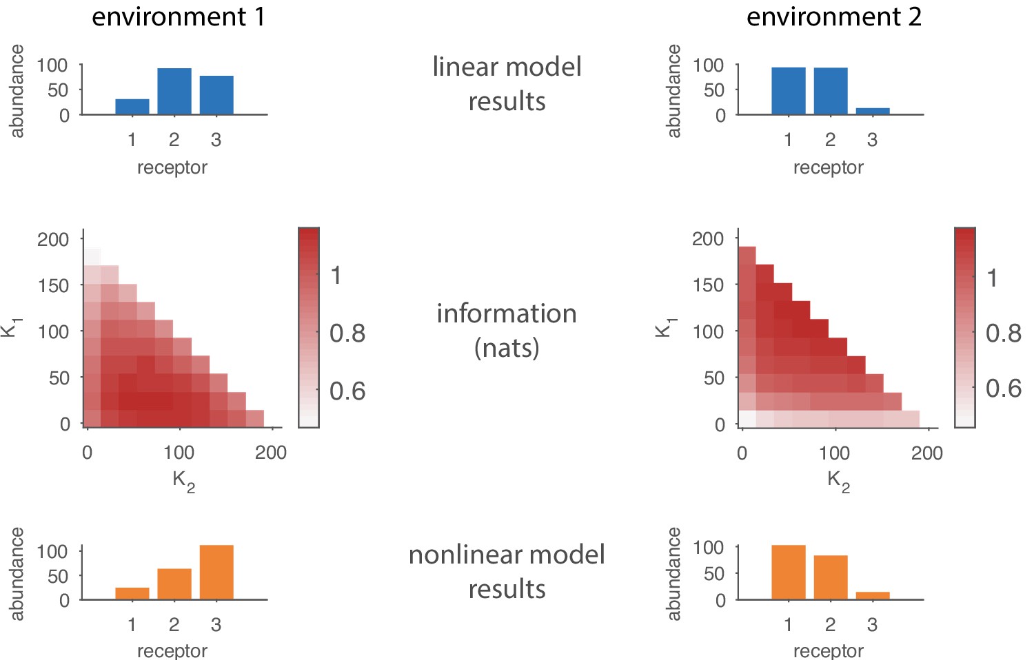
Comparing results from the linear model in the main text to results based on a nonlinear response function.
The top row shows the optimal receptor distribution obtained using the linear model for a system with three receptor types and 15 odorants. The middle row shows how the estimated mutual information varies with OSN abundances in a nonlinear model based on a competitive binding response function. The bottom rows shows the optimal receptor distribution from the nonlinear model, obtained by finding the cells in the middle row in which the information is maximized.
Additional files
-
Transparent reporting form
- https://doi.org/10.7554/eLife.39279.011
Download links
A two-part list of links to download the article, or parts of the article, in various formats.
Downloads (link to download the article as PDF)
Open citations (links to open the citations from this article in various online reference manager services)
Cite this article (links to download the citations from this article in formats compatible with various reference manager tools)
Adaptation of olfactory receptor abundances for efficient coding
eLife 8:e39279.
https://doi.org/10.7554/eLife.39279


