Figures and data in Time preferences are reliable across time-horizons and verbal versus experiential tasks

Figures
Videos
Tables
Additional files

7 figures, 4 videos, 4 tables and 6 additional files

Figures

Figure 1 with 1 supplement

Download asset Open asset

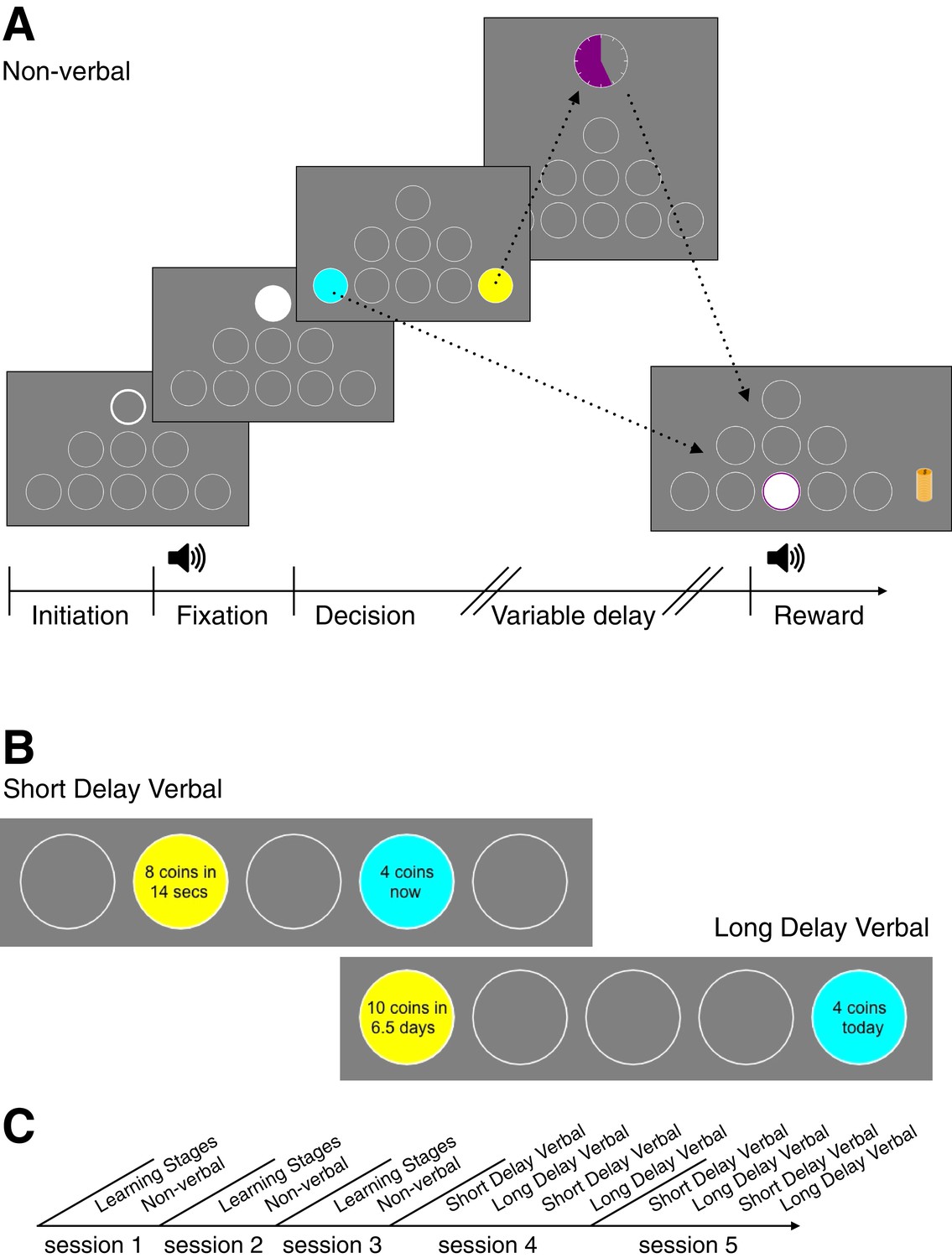
Behavioral Tasks.

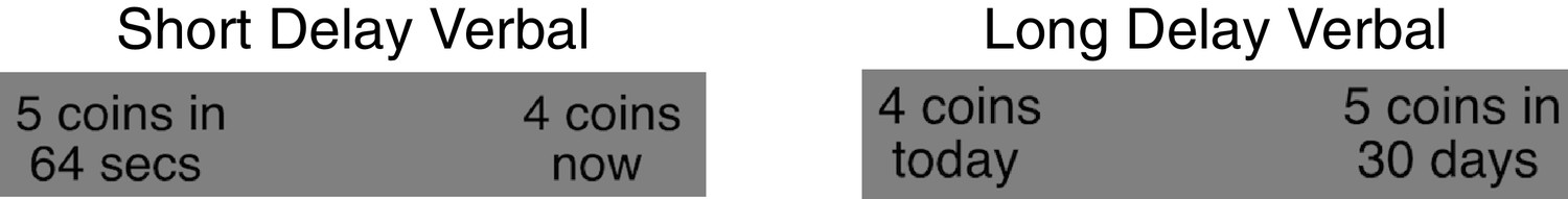
(A) A novel language-free intertemporal choice task. This is an example sequence of screens that subjects viewed in one trial of the non-verbal task. First, the subject initiates the trial by pressing on the white-bordered circle. During fixation, the subject must keep the cursor inside the white circle. The subject hears an amplitude modulated pure tone (the tone frequency is mapped to reward magnitude and the modulation rate is mapped to the delay of the later option). The subject next makes a decision between the sooner (blue circle) and later (yellow circle) options. If the later option is chosen, the subject waits until the delay time finishes, which is indicated by the colored portion of the clock image. Finally, the subject clicks in the middle bottom circle (‘reward port’) to retrieve their reward. The reward is presented as a stack of coins of a specific size and a coin drop sound accompanies the presentation. (B) Stimuli examples in the verbal experiment during decision stage (the bottom row of circles is cropped). (C) Timeline of experimental sessions. Note: The order of short and long delay verbal tasks for sessions 4 and 5 was counter-balanced across subjects.

https://doi.org/10.7554/eLife.39656.002

Figure 1—figure supplement 1

Download asset Open asset

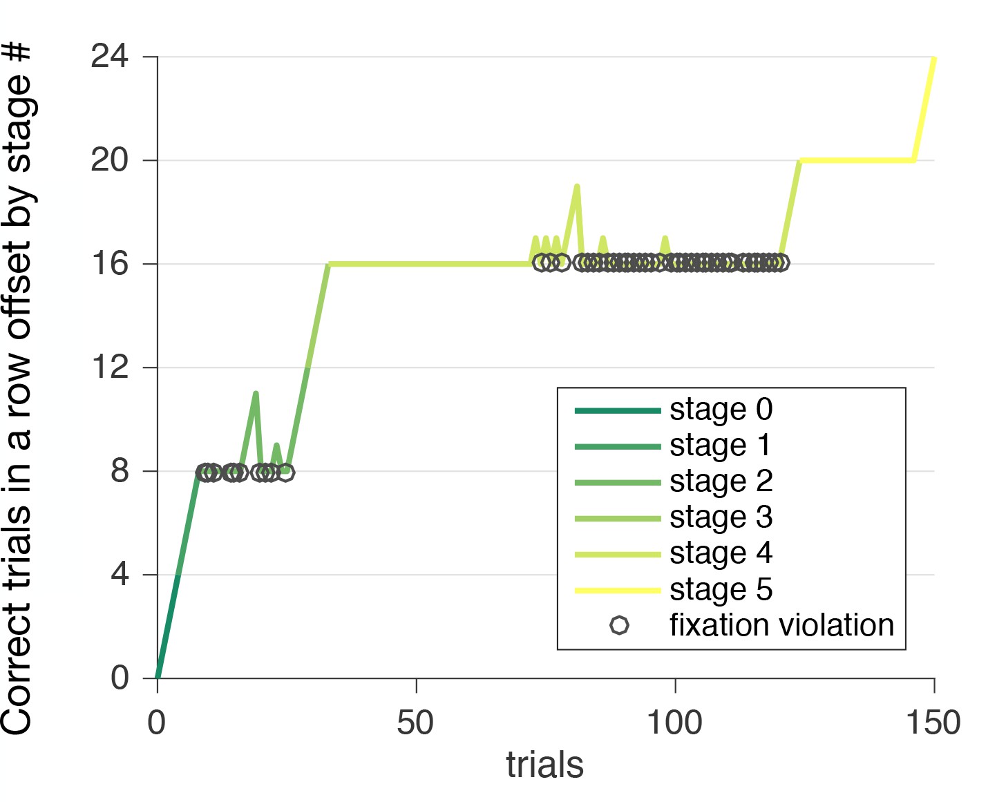
Learning stages example performance.

This figure shows the pattern of correct choices vs. violations made by a single subject. Each one unit increase in y with increase in x (trials) is a correct trial. Each violation drops the ‘correct in a row’ measure to 0 for each stage. Four correct trials in a row are required to advance to the next learning stage. The circles identify fixation violations. Some subjects experienced difficulty with the learning to ‘fixate’ during learning stage 2. Subjects that didn’t pass learning stages stopped at this stage. This is the only stage where the % correct trials was less than 40% compared to more than 70% in other stages. Subjects on average also spent significantly more time for the learning stage two compared to the next learning stage 3 (Wilcoxon signed-rank test, $p < 0.01$ ), although only four trials without violations are required to pass this learning stage and learning stage three includes more steps. Fixation was specifically designed to drive subjects attention away from the computer mouse and to pay attention to the sound. During fixation in the learning stages 4 and 5 (as well as in the decision stages) subjects hear sound that corresponds to the reward magnitude and delay. There were three major patterns of violations across subjects: (1) subject had difficulty passing stage 2 (because of fixation violations), however later stages were completed quickly; (2) subject was able to pass stage 2, by having four correct answers in a row, but during stage four encountered problems with fixation violation again (this pattern is showed in the figure); (3) subject was able to proceed till stage five almost without violations, but was stopped by several fixation violations at stage 5. There were no significant differences between learning stage performance across demographic categories, such as gender and nationality (percent trials without violation, mean $\pm$ std. dev. for females: $0.75 \pm 0.28$ and males: $0.79 \pm 0.27$ , Wilcoxon rank sum test, $p < 0.1$ ; Chinese: $0.75 \pm 0.29$ and Non-Chinese: $0.79 \pm 0.26$ , Wilcoxon rank sum test, $p = 0.13$ )).

https://doi.org/10.7554/eLife.39656.003

Figure 2 with 4 supplements

Download asset Open asset

A 50% median split (±1 standard deviation) of the softmax-hyperbolic fits.

(**A–C**) more patient and (**D–F**) less patient subjects. The values of $k$ and $τ$ are the means within each group. Average psychometric curves obtained from the model fits (lines) versus actual data (circles with error bars) for NV, SV and LV tasks for each delay value, where the x-axis is the reward magnitude and the y-axis is the probability (or proportion for actual choices) of later choice. Error bars are binomial 95% confidence intervals. We excluded the error in the model for visualization. Note: The lines here are not a model fit to aggregate data, but rather reflect the mean model parameters for each group. As such, discrepancies between the model and data here are not diagnostic. See individual subject plots (Supplementary file 1) to visualize the quality of the model fits.

https://doi.org/10.7554/eLife.39656.004

Figure 2—figure supplement 1

Download asset Open asset

An example of the softmax-hyperbolic fit for one subject in Matlab and Stan.

This figure shows an example of the softmax-hyperbolic fit for one subject. (**A–C**) Matlab fits, (**D–F**) BHM fits. Psychometric curves obtained from the model fits versus actual data (circles) for non-verbal (NV) and verbal (short (SV) and long (LV) delay) tasks for each delay value, where the x-axis is the reward and the y-axis is the probability (or proportion for actual choices) of later choice. Error bars reflect 95% binomial confidence intervals. We can readily observe that although first-order violations were present during non-verbal task, in the verbal task they get eliminated. Also whereas the unit-free discount rates seem pretty stable, the decision noise $τ_{i}$ gets smaller from non-verbal to verbal tasks. The roles of different parameters in softmax-hyperbolic fit are well shown in (Figure 2—figure supplement 4).

https://doi.org/10.7554/eLife.39656.005

Figure 2—figure supplement 2

Download asset Open asset

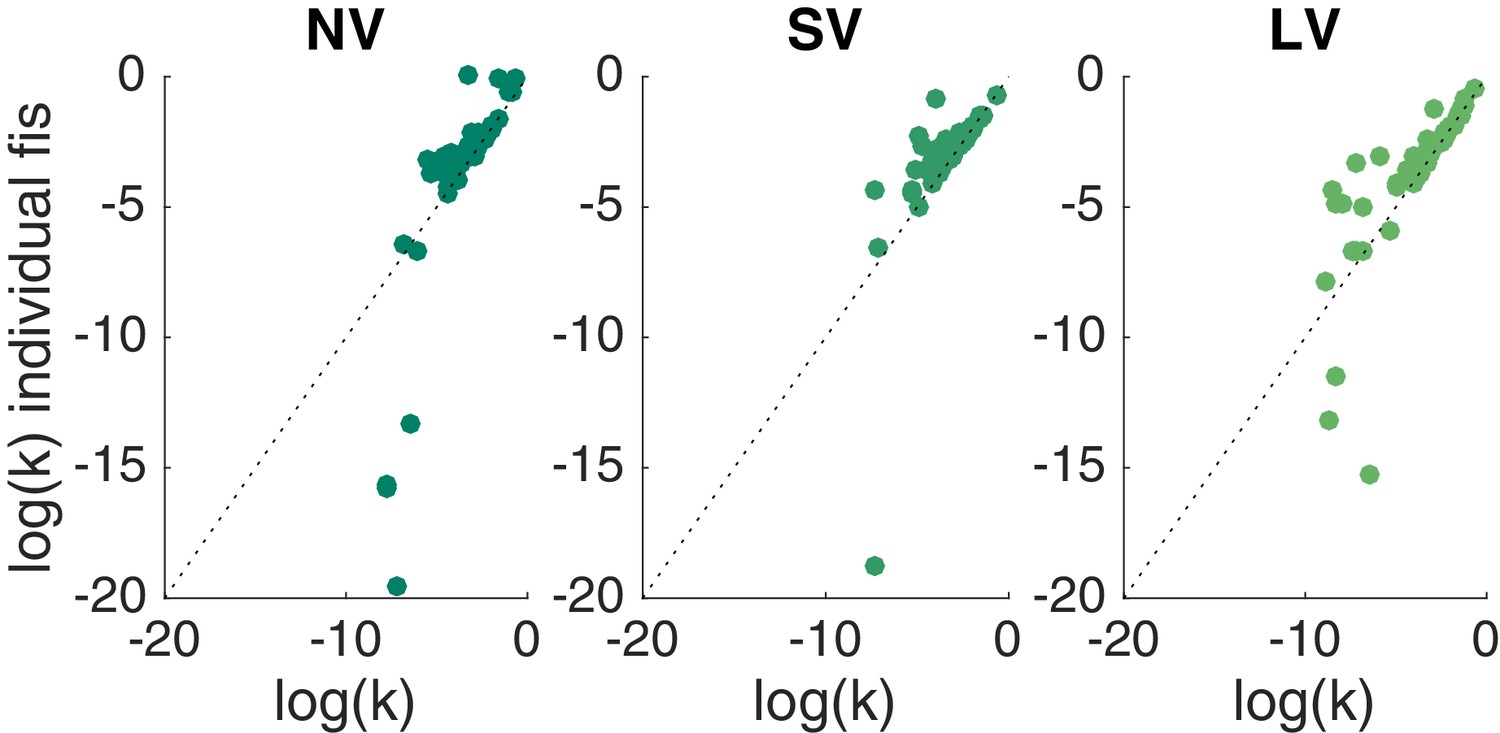
BHM fits vs. Matlab fits.

BHM model fits (x-axis) vs. Matlab individual data fits (y-axis) across tasks against the unity line. Since the estimation procedure was identical for all MLE fits (Matlab code is available on github repository), we describe it using the softmax-hyperbolic model as an example. This is a two-parameter model to estimate choice behavior, that is, it transforms the stimulus on each trial (inputs to the model include rewards and delays for sooner and later options) into a probability distribution about the subject’s choice. For example, if for a given set of parameters, the model predicts that trial one will result in 80% chance of the subject choosing later option, and the subject, in fact, chose the later, the trial would be assigned a likelihood of 0.8 (if the subject chose sooner, the trial would have a likelihood of 0.2). Finally, we perform a leave-one-out cross-validation for each subject-task to avoid overfitting. We leave one trial out and use the rest of the trials in the experimental task to predict this trial. We repeat this procedure for each trial. Instead of getting point estimates (or distributions of parameter values through cross-validation as we did) one can use a Bayesian hierarchical model (BHM, estimation details in Materials and methods) to find full posterior distributions. It allows for both pooling data across subjects and recognizing individual differences. The fits from BHM model are almost identical to the individual fits done for each experimental task separately using softmax-hyperbolic model and ‘fmincon’ function in Matlab. The exceptions are very patient subjects that almost exclusively picked the later option. For these subjects, the MLE fits can produce discount factors $< e^{- 10}$ , but the prior in the BHM model constrains these to be around $e^{- 8}$ . Furthermore, the rank correlation values for MLE fits correspond to the BHM ones both in magnitude and significance. Rank correlations obtained from individual level MLE fits for top three models by BIC: (NV vs. SV) Spearman $r$ = 0.52, 0.68, 0.38 for hyperbolic utility with matching rule, hyperbolic utility with softmax and exponential utility with softmax models, respectively; (SV vs. LV) Spearman $r$ = 0.46, 0.49, 0.5, all $p < 0.01$ .

https://doi.org/10.7554/eLife.39656.006

Figure 2—figure supplement 3

Download asset Open asset

Non-parametric out-of-sample prediction.

To validate our model-free analysis we did a non-parametric out-of-sample prediction by summarizing each subject’s choices into a 7-D vector (based on delay and reward) for each task ( $3 \times 7 = 21$ -D total). Each 7-D vector was constructed by taking the fraction of delayed choices for [‘small’ rewards (1 or 2 coins), ‘medium’ reward and ‘small’ delay (5 coins in 3 or 6.5 s/days), ‘medium’ reward and ‘medium’ delay (5 coins in 14 s/days), ‘medium’ reward and ‘large’ delay (5 coins in 30 or 64 s/days), ‘large’ reward and ‘small’ delay (8 or 10 coins in 3 or 6.5 s/days), ‘large’ reward and ‘medium’ delay (8 or 10 coins in 14 s/days), ‘large’ reward and ‘large’ delay (8 or 10 coins in 30 or 64 s/days)]. Having summarized each subject as a 21-D vector, we performed a leave-one-subject/task-out cross-validation. For each subject-task, we trained a linear model to predict the choices from one task (e.g. the 7-D vector for SV) based on the other two tasks (the 14-D vector of NV and LV) for all subjects (other than the left out subject). Then, for the left out subject, we predicted each task from the other two. We can predict 68% of the subjects 21-vectors this way. We conclude that, for most subjects, there is a shared scaling effect that allows each tasks’ choices to be predicted by the other two. This figure shows the distribution of the Pearson correlation coefficients between real and predicted 21-vectors of each subject. Darker bars are significant correlations.

https://doi.org/10.7554/eLife.39656.007

Figure 2—figure supplement 4

Download asset Open asset

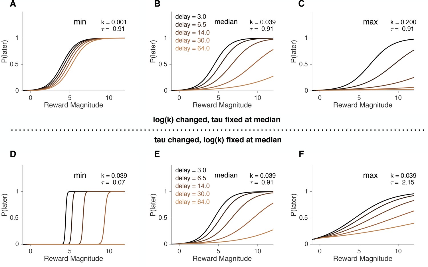
The role of parameters in hyperbolic utility model with softmax.

To illustrate how model parameters affect predicted choices, we simulated choices of softmax-hyperbolic ‘agents’ for specific values of discount factor, $k$ , and decision noise, $τ$ . (**A–C**) simulated agents that match discount factors of the patient, average and impulsive subjects with $τ$ fixed at the median. (**D–F**) simulations for low, median and high values of $τ$ with $\log (k)$ fixed at the median.

https://doi.org/10.7554/eLife.39656.008

Figure 3 with 4 supplements

Download asset Open asset

Comparison of discount factors across three tasks in the main experiment.

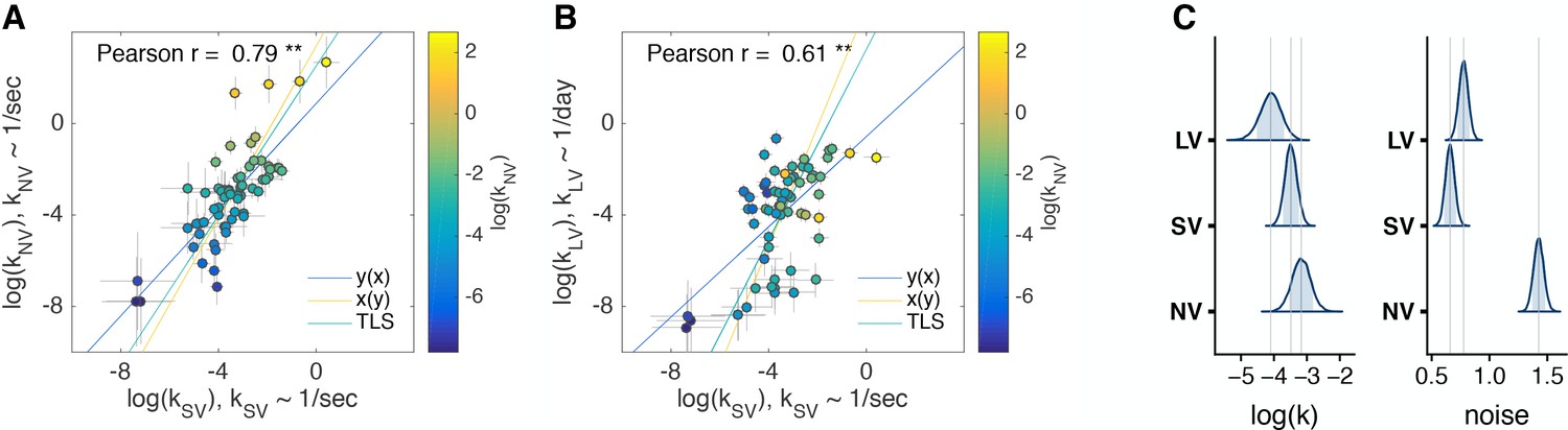
(**A, B**) Each circle is one subject (N = 63). The logs of discount factors in SV task (x-axis) plotted against the logs of discount factors in NV (A) and LV (B) tasks (y-axis). The color of the circles and the colorbar identify the ranksdiscount factors in NV task. Pearson’s $r$ is reported on the figure ( $p < 0.01$ - ’**’). The error bars are the SD of the estimated coefficients (posterior means). Three lines (Huang et al., 2013) represent the vertical $y (x)$ , horizontal $x (y)$ and perpendicular (or total) least squares (TLS) regression lines. (C) Distribution of posterior parameter estimates of $\log (k)$ and decision noise $τ$ from the model fit for the three tasks in the main experiment ( $k_{N V} \sim 1 / \sec$ , $k_{S V} \sim 1 / \sec$ , $k_{L V} \sim 1 / d a y$ ). The light blue shaded area marks the 80% interval of the posterior estimate. The outline of the distribution extends to the 99.99% interval. Thin grey lines are drawn through the mean of each distribution to ease comparison across tasks. Comparisons between tasks are reported in Table 3. Note, the units for $k_{S V}$ & $k_{N V}$ ( $1 / \sec$ ) would need to be scaled by $86400 s e c s / d a y \to \log (86400) = 11.37$ to be directly compared to $k_{L V}$ .

https://doi.org/10.7554/eLife.39656.009

Figure 3—figure supplement 1

Download asset Open asset

Model-free analysis of short tasks.

Additional model-free measures of discounting behavior are correlated with the discount factors estimated using BHM model. Each dot is one subject from the main experiment. (**A, B**) Total time spent per task (x-axis) plotted against fraction of total reward (y-axis) shows significant positive relationship (NV: Pearson $r = 0.82$ , $p < 0.01$ ; SV: Pearson $r = 0.90$ , $p < 0.01$ ). The more you wait (the more you spend time for the session), the more you earn, unless you make first-order violations by choosing later offers that are worse than the immediate option. (**C, D**) The logs of discount factors (x-axis) plotted against the fraction of total reward (y-axis) result in significant negative correlations for NV (Pearson $r = - 0.93$ , $p < 0.01$ ) and SV (Pearson $r = - 0.92$ , $p < 0.01$ ). (**E, F**) The logs of discount factors (x-axis) plotted against the non-waiting time (total task time minus waiting time, y-axis). In NV Pearson $r = - 0.28$ , $p < 0.05$ and SV Pearson $r = - 0.64$ , $p < 0.01$ . Similar significant relationship is also observed for the $\log (k)$ and waiting time (not plotted, NV: Pearson $r = - 0.84$ , $p < 0.01$ ; SV: Pearson $r = - 0.92$ , $p < 0.01$ ). What is important, across subjects non-waiting time is significantly correlated with waiting time, meaning that impulsive subjects were also quick in everything else (reaction time, mouse movement and clicks, NV: Pearson $r = 0.32$ , $p < 0.05$ ; SV: Pearson $r = 0.66$ , $p < 0.01$ ). (**G, H, I**) Significant negative relationship of the logs of discount factors (x-axis) with the total time (total time spent on a task, y-axis) in the NV (Pearson $r = - 0.81$ , $p < 0.01$ ) and SV (Pearson $r = - 0.91$ , $p < 0.01$ ), but not LV (Pearson $r = 0.17$ , $p = 0.19$ ).

https://doi.org/10.7554/eLife.39656.010

Figure 3—figure supplement 2

Download asset Open asset

Ruling out the anchoring effect.

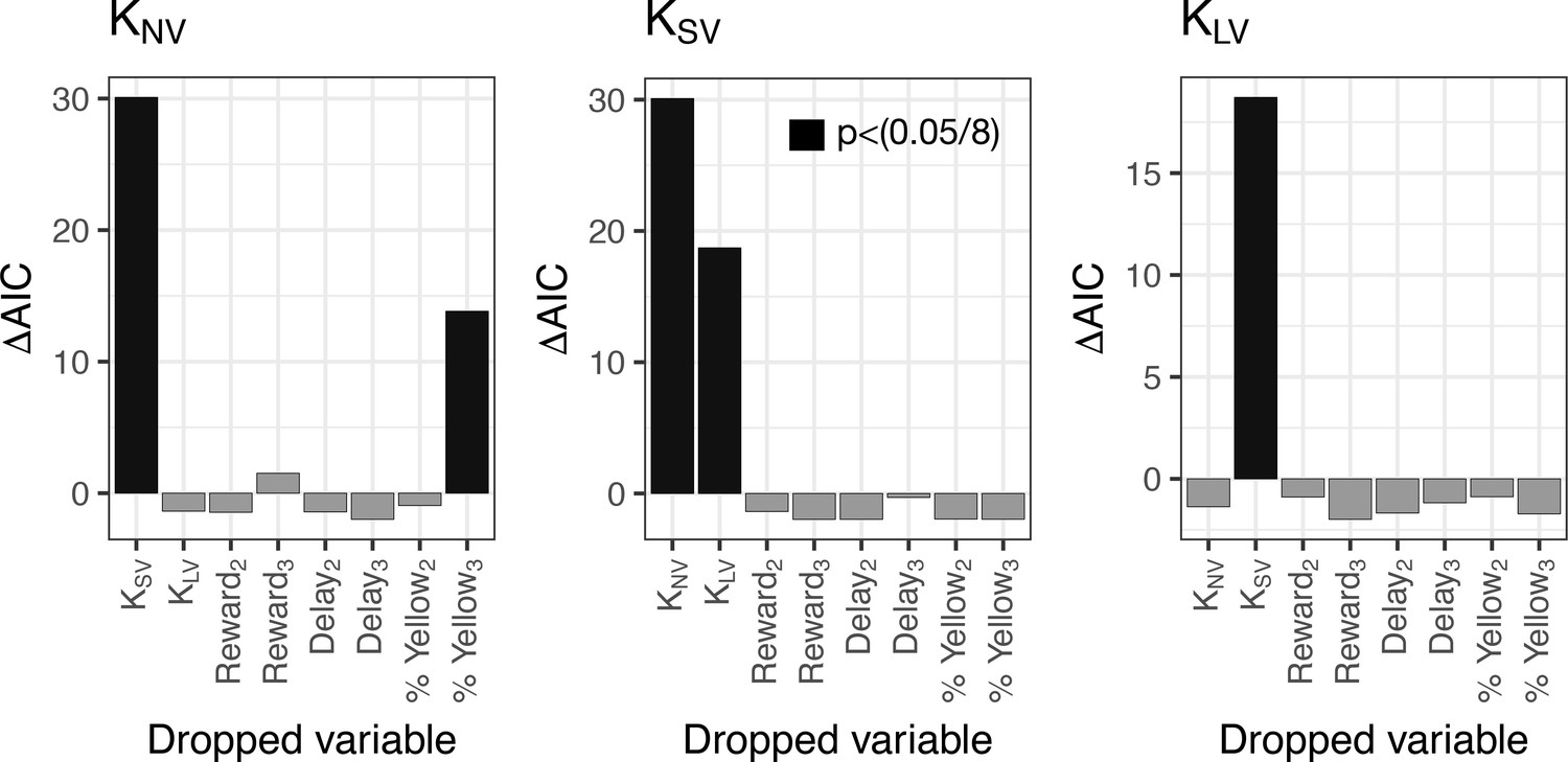
Analysis of the source of correlation in discount-factor across tasks. We generated linear regression models of $\log (k)$ for each task against the discount factors of the other tasks, as well as reward, delay and % of yellow choices of the first reward block in NV task. In order to test which factors were important, we dropped each factor and tested the whether the decrease in likelihood was significant a Chi Squared test. (Analyses were done in R using the ‘drop1’ function). We plot the change in AIC, where significant ( $p < 0.00625$ , Bonferroni Corrected $p < 0.05 / 8$ ) drops are in black. The subscript $2$ or $3$ in dropped variables is used to identify whether the first block comes from NV session 2 or 3, respectively.

https://doi.org/10.7554/eLife.39656.011

Figure 3—figure supplement 3

Download asset Open asset

Obtained subjective utilities and hyperbolic fits of individual subjects.

Individual subjects fits and subjective utilities as a function of the delay in units of the task ordered by log of discount factor for SV. Three subjects were picked to represent 10%, 50% and 90% percentiles of $\log (k_{S V})$ . Solid curves show the subjective utility of a 5 coins reward discounted by subjects. The dotted curve represent the subjective utility of a 10 coins reward discounted by subjects.

https://doi.org/10.7554/eLife.39656.012

Figure 3—figure supplement 4

Download asset Open asset

Simulation results: distributions of expected correlations of the discount factors ranks between tasks.

Given that we are estimating subjects discount-factors using a finite number of trials per task, even if subjects’ discount-factors were identical in different tasks, we would not expect the rank correlations to be perfect. In order to estimate the expected maximum correlation we could observe, we simulated ‘consistent’ subjects’ choices using hyperbolic model with softmax rule, assuming that there is a single delay-discounting parameter, $k_{i}$ , (mean across tasks) for each subject. We did this 100,000 times and computed a distribution of pairwise rank correlations. These simulations revealed that the decision noise contributed a very small amount of variance.

https://doi.org/10.7554/eLife.39656.013

Figure 4 with 1 supplement

Download asset Open asset

Comparison of discount factors across three tasks in control experiment 1.

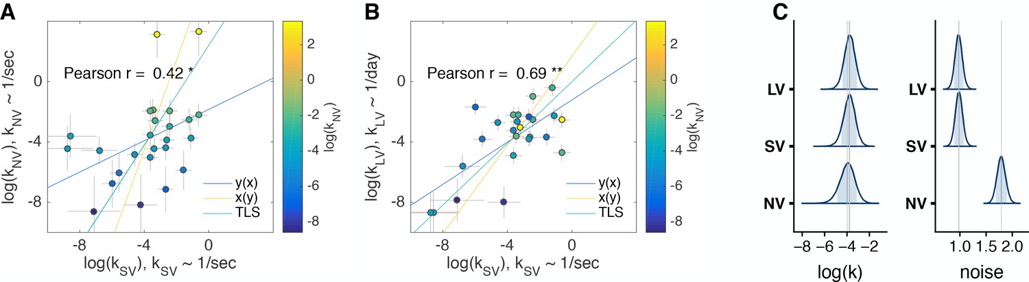
(**A,B**) Control experiment 1 (n = 25). The logs of discount factors in SV task (x-axis) plotted against the logs of discount factors in NV (A) and LV (B) tasks (y-axis). The color of the circles and the colorbar identify the discount factors in NV task. Each circle is one subject. Pearson’s $r$ is reported on the figure ( $p < 0.01$ - ‘**’, $p < 0.05$ - ‘*’). Spearman $r$ : SV vs. NV $r = 0.52$ ; SV vs. LV $r = 0.52$ (all $p < 0.01$ ). The error bars are the SD of the estimated coefficients. Three lines represent the vertical $y (x)$ , horizontal $x (y)$ and total least squares (TLS) regression lines. See individual subject plots (Supplementary file 2) to visualize the quality of the model fits. (C) Distribution of posterior parameter estimates of $\log (k)$ and decision noise $τ$ from the model fit for the three tasks in control experiment 1 ( $k_{N V} \sim 1 / s$ , $k_{S V} \sim 1 / s$ , $k_{L V} \sim 1 / d a y$ ). The light blue shaded area marks the 80% interval of the posterior estimate. The outline of the distribution extends to the 99.99% interval. Thin grey lines are drawn through the mean of each distribution to ease comparison across tasks.

https://doi.org/10.7554/eLife.39656.017

Figure 4—figure supplement 1

Download asset Open asset

Control experiment 1 choice screen example.
https://doi.org/10.7554/eLife.39656.018

Figure 5

Download asset Open asset

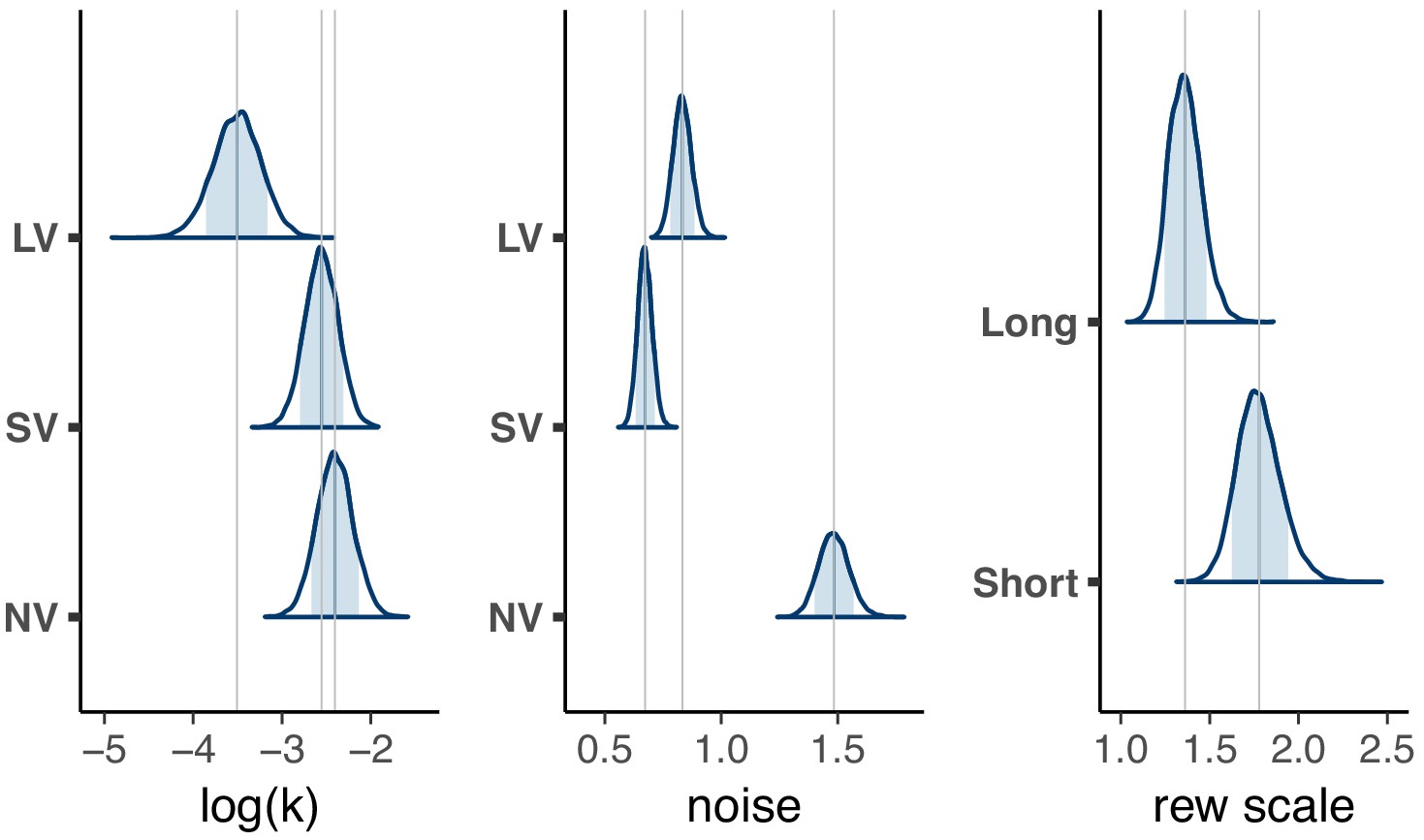
Distribution of population level posterior parameter estimates from the expanded model fit with reward scaling for the three tasks in the main experiment.

The light blue shaded area marks the 80% interval of the posterior estimate. The outline of the distribution extends to the 99.99% interval. Thin grey lines are drawn through the mean of each distribution to ease comparison across tasks. Note, the units for $k_{S V}$ & $k_{N V}$ ( $1 / s$ ) would need to be scaled by $86400 s e c s / d a y \to \log (86400) = 11.37$ to be directly compared to $k_{L V} (1 / d a y)$ .

https://doi.org/10.7554/eLife.39656.019

Figure 6 with 1 supplement

Download asset Open asset

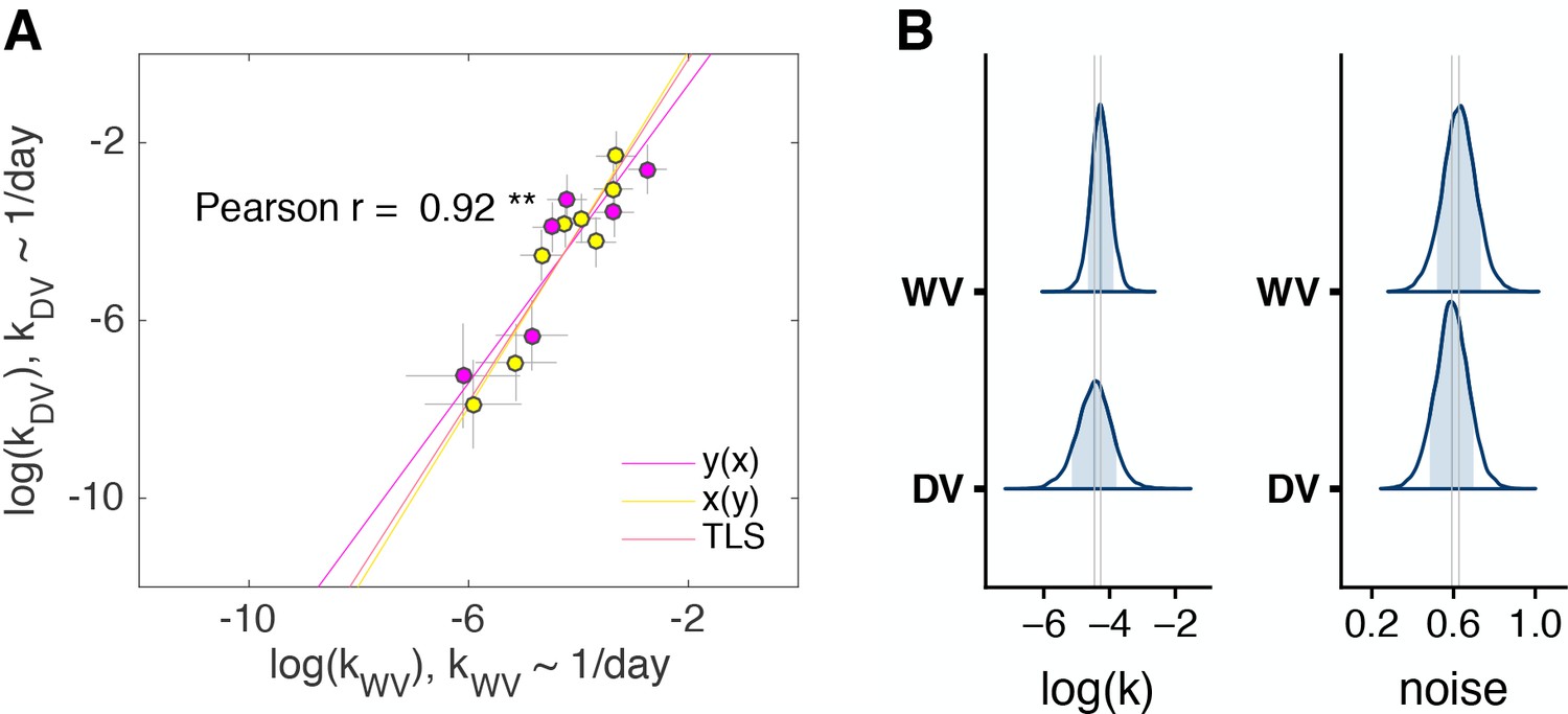
Control experiment 2.

(A) The discount factors in WV task plotted against the discount factors in DV task, (n = 14, two out of 16 subjects who always chose the later option were excluded from the model). The color of the circles identifies the order of task appearance. Each circle is one subject. Pearson’s $r$ is reported on the figure ( $p < 0.01$ - ‘**’). The error bars are the SD of the estimated coefficients. Three lines represent the vertical $y (x)$ , horizontal $x (y)$ and total least squares (TLS) regression lines. See individual subject plots (Supplementary file 3) to visualize the quality of the model fits. (B) Distribution of posterior parameter estimates of $\log (k)$ and decision noise $τ$ from the model fit for the two tasks in control experiment 2 ( $k_{D V} \sim 1 / d a y$ , $k_{W V} \sim 1 / d a y$ ). The light blue shaded area marks the 80% interval of the posterior estimate. The outline of the distribution extends to the 99.99% interval. Thin grey lines are drawn through the mean of each distribution to ease comparison across tasks.

https://doi.org/10.7554/eLife.39656.021

Figure 6—figure supplement 1

Download asset Open asset

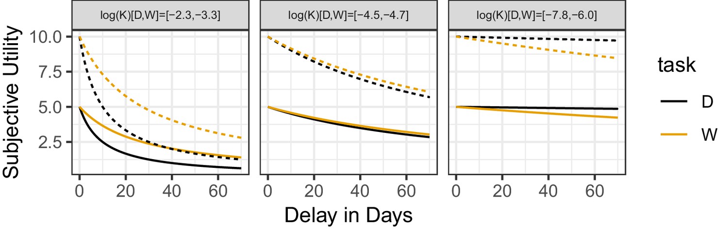
Subjective utilities as a function of the delay in days.

Control experiment 2. Subjective utilities as a function of the delay in days and hyperbolic fits of individual subjects. Left to right panels are ordered by log of discount factor for SV. Three subjects were picked to represent 10%, 50% and 90% percentiles of $\log (k_{S V})$ . Solid line shows the subjective utility of a 5 coins reward discounted by subjects. The dotted line shows the subjective utility of a 10 coins reward discounted by subjects. Discount factors for all tasks for each example subject are displayed above each panel.

https://doi.org/10.7554/eLife.39656.022

Figure 7

Download asset Open asset

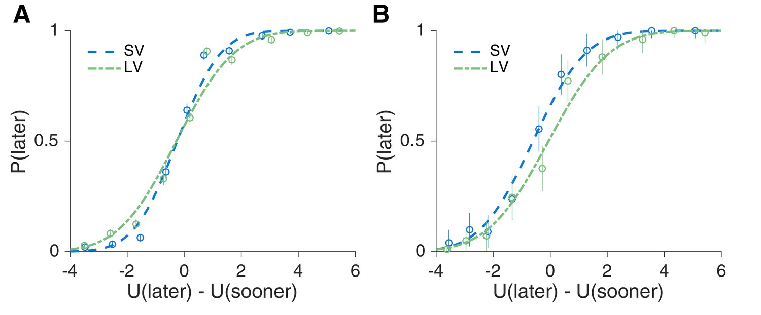
Evidence for context dependent temporal processing.

(**A,B**) Main experiment early trials adaptation effect. The offers for each subject were converted into a subjective utility, U, based on the subjects’ discount factors in each task. This allowed us to combine data across subjects to plot psychometric curves of the probability of choosing the later option, $P (l a t e r)$ , for SV and LV averaged across all subjects comparing late trials (Trial in task > 5) (A) to the first four trials (B). Using a generalized linear mixed effects model, we found a significant interaction between *early/late* and *SV/LV* ( $β_{S V L V : e a r l y} = 0.86 \pm 0.17, p < 10^{- 6}$ , $n_{s u b j e c t s} = 63, n_{t r i a l s} = 20387$ ).

https://doi.org/10.7554/eLife.39656.023

Videos

Video 1

Download asset

posterframe for video — Learning.

A video of the learning stages, showing the examples of violations that can be made. The video starts with stage 0 and continues with stage 1 at 00:14, stage 2 at 00:31, stage 3 at 00:55, stage 4 (trimmed) at 01:18 and stage 5 (trimmed) at 01:41.

https://doi.org/10.7554/eLife.39656.024

Video 2

Download asset

Video 3

Download asset

Video 4

Download asset

Tables

Table 1

Correlations of subjects’ discount factors [95% CI].

Corrected rank correlations of subjects’ discount factors were normalized using simulations to estimate the expected maximum correlation we could observe (Figure 3—figure supplement 4). The correlations between each task were significantly different from each other at $p < 0.05$ using various methods as in the R package ‘cocor’ (Diedenhofen and Musch, 2015).

https://doi.org/10.7554/eLife.39656.014

	Spearman Rank Correlation	Corrected Rank Correlation	Pearson Correlation
SV vs. NV	0.76 [0.61, 0.85]	0.77 [0.62, 0.87]	0.79 [0.65, 0.88]
SV vs. LV	0.54 [0.30, 0.73]	0.57 [0.31, 0.77]	0.61 [0.41, 0.76]
NV vs. LV	0.36 [0.11, 0.57]	0.39 [0.12, 0.62]	0.40 [0.18, 0.60]

all $p < 0.01$

Table 2

Relative contributions of two gaps to variance in $\log (k)$ (two-factor model comparison with two reduced one-factor models).

https://doi.org/10.7554/eLife.39656.015

Dropped factor	$Δ d f$	AIC	LR test $p$
none		743.06
verbal	1	742.88	0.18
days	1	745.99	0.03

Table 3

Shift and scale of $\log (k)$ between tasks.

$k_{S V}, k_{N V} \sim (1 / s)$ . $k_{L V} \sim (1 / d a y)$ . The evidence ratio (Ev. Ratio) is the Bayes factor of a hypothesis vs. its alternative, for example $P (a > b) / P (a < b)$ . '*’denotes $p < 0.01$ , one-sided test. Expressing $\log (k_{L V})$ in units of 1/s (for direct comparison with the other tasks) results in a negative shift in $\log (k_{L V})$ and even larger differences in means without changing the difference between standard deviations.

https://doi.org/10.7554/eLife.39656.016

Comparison	$l o g_{2} (E v . R a t i o)$
between means
$μ \log (k_{S V}) > μ \log (k_{L V})$	6.79 *
$μ \log (k_{N V}) > μ \log (k_{L V})$	7.92 *
$μ \log (k_{N V}) > μ \log (k_{S V})$	4.16
between standard deviations
$σ \log (k_{L V}) > σ \log (k_{S V})$	8.43 *
$σ \log (k_{N V}) > σ \log (k_{L V})$	0.92
$σ \log (k_{N V}) > σ \log (k_{S V})$	11.48 *

Table 4

Correlations of subjects’ log discount factors [95% CI] in the original model (taken from Table 1) and the expanded model which included differential reward scaling between the short and long tasks.

The correlations between each task were significantly different from each other at $p < 0.05$ for both the original and expanded models using various methods as in the R package ‘cocor’ (Diedenhofen and Musch, 2015).

https://doi.org/10.7554/eLife.39656.020

	Original model Pearson Correlation	Expanded model Pearson Correlation
SV vs. NV	0.79 [0.65, 0.88]	0.84 [0.75, 0.90]
SV vs. LV	0.61 [0.41, 0.76]	0.65 [0.48, 0.77]
NV vs. LV	0.40 [0.18, 0.60]	0.50 [0.29, 0.66]

all correlations are significantly different from 0, $p < 0.01$

Additional files

Supplementary file 1 Individual subjects fits for main experiment. Each plot is the softmax-hyperbolic fit for each subject in the main experiment. In each panel, the marker and error bar indicate the mean and binomial confidence intervals of the subjects choices for that offer. The smooth ribbon indicated the BHM model fits (at 50, 80, 99% credible intervals). At the top of each subject plot we indicate the mean estimates of $\log (k)$ and $τ$ for each task for that subject. We also indicate the Bayesian $r^{2}$ for each task. Plots from Left to right, row-by-row are ordered by discount factor (as estimated using BHM) for SV.: https://doi.org/10.7554/eLife.39656.029
Download elife-39656-supp1-v1.pdf
Supplementary file 2 Individual subjects fits for control experiment 1. Each plot is the softmax-hyperbolic fit for each subject in the control experiment 1. In each panel, the marker and error bar indicate the mean and binomial confidence intervals of the subjects choices for that offer. The smooth ribbon indicated the BHM model fits (at 50, 80, 99% credible intervals). At the top of each subject plot we indicate the mean estimates of $\log (k)$ and $τ$ for each task for that subject. We also indicate the Bayesian $r^{2}$ for each task. Plots from Left to right, row-by-row are ordered by discount factor for SV.: https://doi.org/10.7554/eLife.39656.030
Download elife-39656-supp2-v1.pdf
Supplementary file 3 Individual subjects fits for control experiment 2. Each plot is the softmax-hyperbolic fit and data for each subject in control experiment 2. In each panel, the marker and error bar indicate the mean and binomial confidence intervals of the subjects choices for that offer. The smooth ribbon indicated the BHM model fits (at 50, 80, 99% credible intervals). At the top of each subject plot we indicate the mean estimates of $\log (k)$ and $τ$ for each task for that subject. We also indicate the Bayesian $r^{2}$ for each task. Plots from Left to right, row-by-row are ordered by discount factor for SV.: https://doi.org/10.7554/eLife.39656.031
Download elife-39656-supp3-v1.pdf
Supplementary file 4 Subject Instructions for non-verbal task.: https://doi.org/10.7554/eLife.39656.032
Download elife-39656-supp4-v1.pdf
Supplementary file 5 Subject Instructions for verbal tasks.: https://doi.org/10.7554/eLife.39656.033
Download elife-39656-supp5-v1.pdf
Transparent reporting form: https://doi.org/10.7554/eLife.39656.034
Download elife-39656-transrepform-v1.docx