Reduced signal for polygenic adaptation of height in UK Biobank
- Columbia University, United States
- Stanford University, United States
- University of Copenhagen, Denmark
- University of California, Davis, United States
- Howard Hughes Medical Institute, Stanford University, United States
Figures
Figure 1 with 1 supplement

Polygenic scores across Eurasian populations, for different GWAS datasets.
The top row shows European populations from the combined 1000 Genomes plus Human Origins panel, plotted against latitude, while the bottom row shows all Eurasian populations from the same combined dataset, plotted against longitude.
Figure 1—figure supplement 1
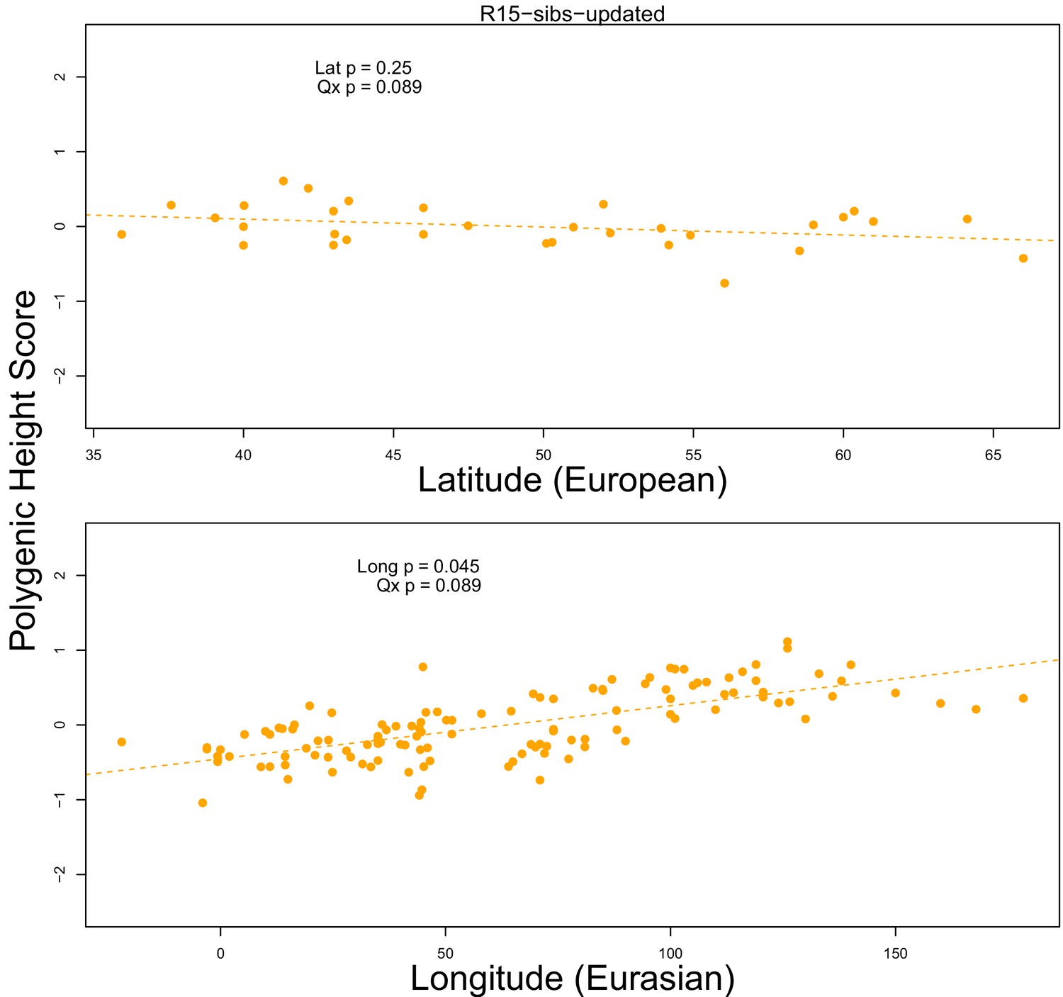
The R15-sibs-updated dataset shows no significant latitudinal or longitudinal signal.
Top Panel: European polygenic scores computed from 1700 smallest p-value SNPs across approximately independent linkage blocks in the R15-sibs-updated dataset, plotted against latitude. Bottom Panel: Eurasian polygenic scores from the same SNP set, plotted against longitude.
Figure 2 with 1 supplement
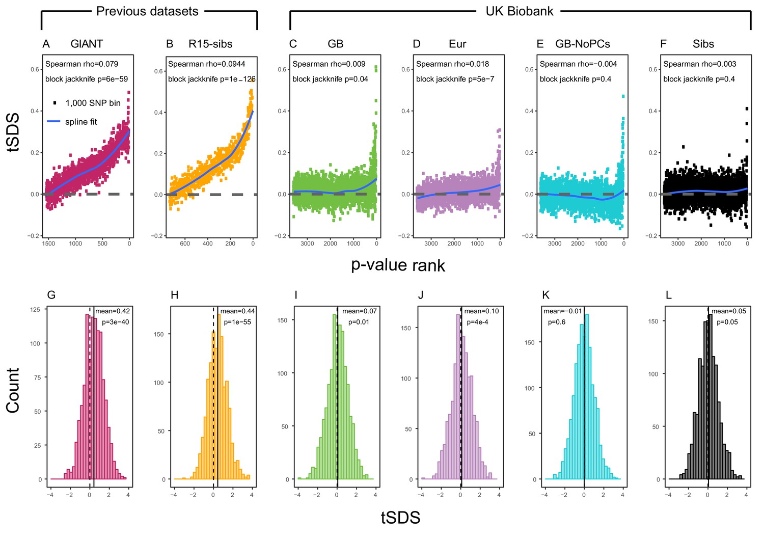
SDS signals for recent selection, assessed using different height GWAS.
(A–F) Each point shows the average tSDS (SDS polarized to height-increasing allele) of 1000 consecutive SNPs in the ordered list of GWAS p-values. Positive values of tSDS are taken as evidence for selection for increased height, and a global monotonic increase—as seen in panels A and B—suggests highly polygenic selection. (G–L) tSDS distribution for the most significant SNPs in each GWAS, thinned according to LD to represent approximately independent signals. Dashed vertical lines show tSDS = 0, as expected under the neutral null; solid vertical lines show mean tSDS. A significantly positive mean value of tSDS suggests selection for increased height.
Figure 2—figure supplement 1
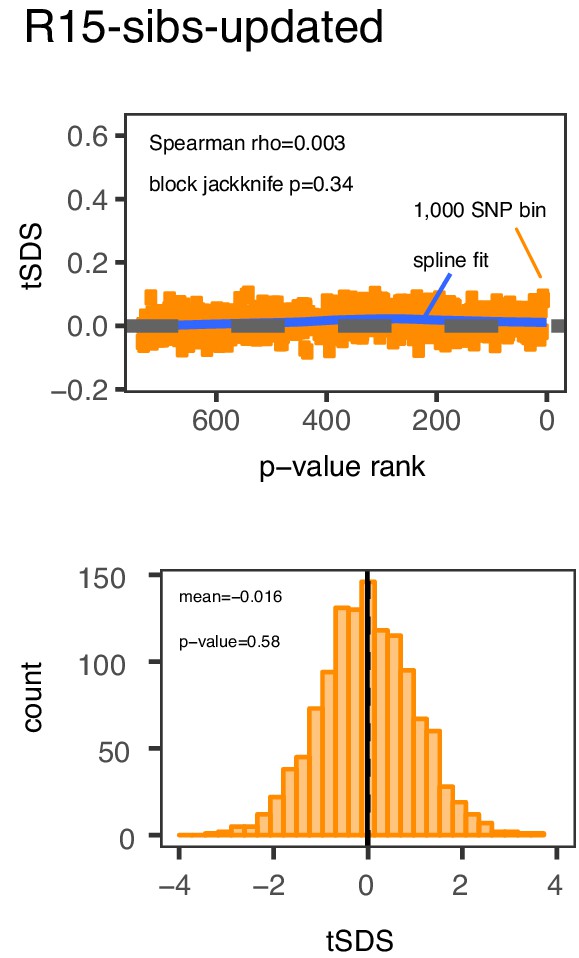
Previously reported SDS selection signals are also absent from the R15-sibs-updated dataset.
Top Panel: SNPs are sorted by p-value in the R15-sibs-updated dataset and then average tSDS is calculated within bins of 1,000 SNPs. Bottom Panel: The distribution of tSDS for 1700 smallest p-value SNPs across approximately independent linkage blocks in the R15-sibs-updated dataset.
Figure 3 with 2 supplements
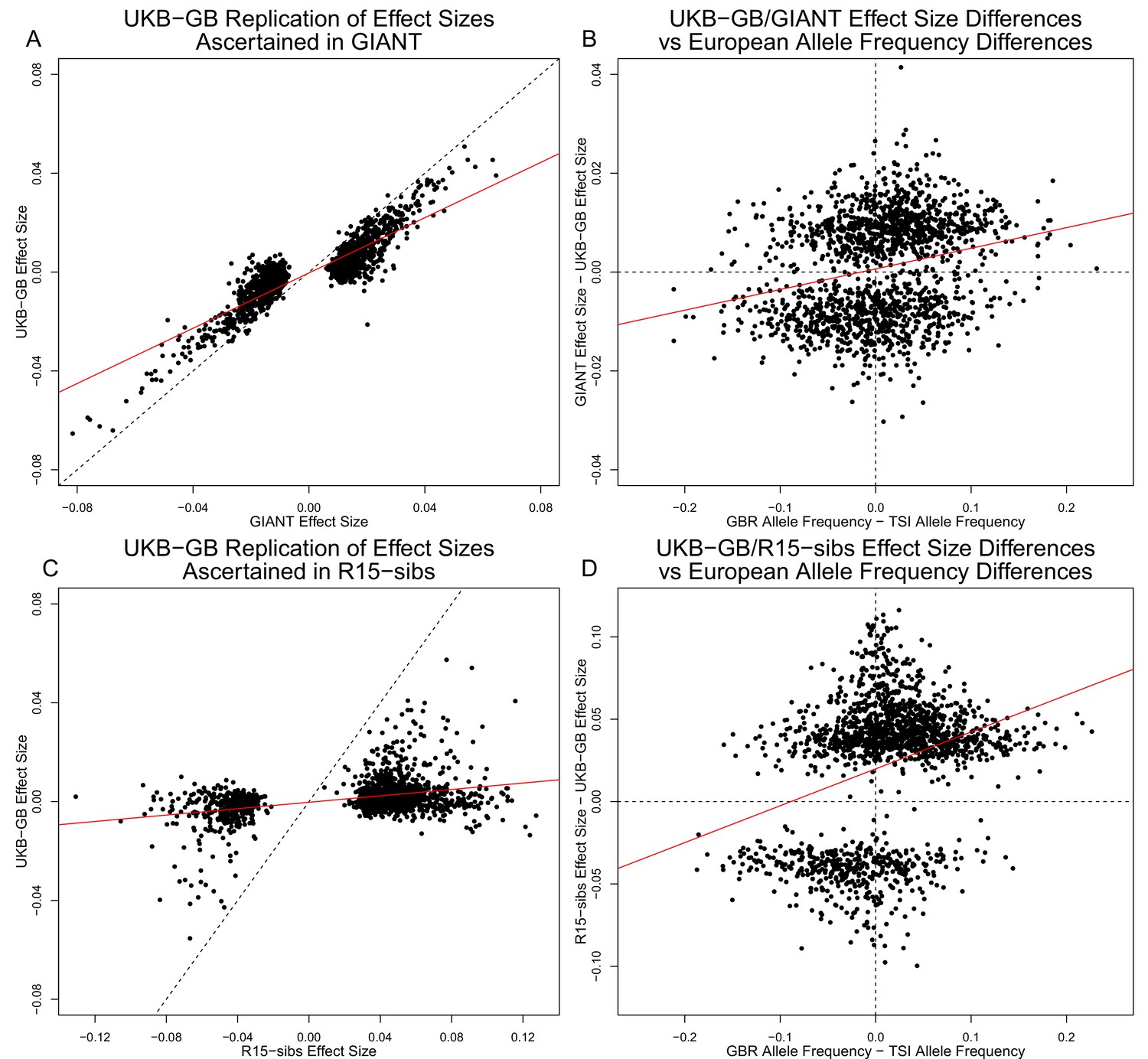
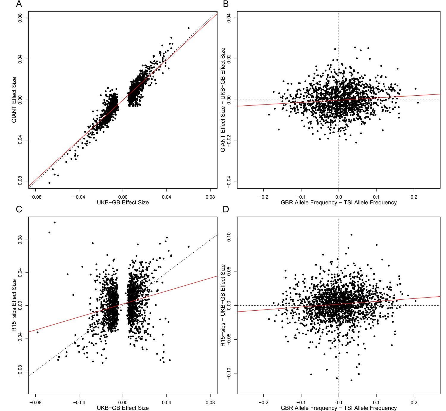
Effect size estimates and population structure.
Top Row: SNPs ascertained using GIANT compared with UKB-GB. (A) The x- and y-axes show the estimated effect sizes of SNPs in GIANT and in UKB-GB. Note that the signals are highly correlated overall, indicating that these partially capture a shared signal (presumably true effects of these SNPs on height). (B) The x-axis shows the difference in ancestral allele frequency for each SNP between 1000 Genomes GBR and TSI; the y-axis shows the difference in effect size as estimated by GIANT and UKB-GB. These two variables are significantly correlated, indicating that a component of the difference between GIANT and UKB-GB is related to the major axis of population structure across Europe. Bottom Row: SNPs ascertained using R15-sibs compared with UKB-GB. (C) The same plot as panel (A), but ascertaining with and plotting R15-sibs effect sizes rather than GIANT. Here, the correlation between effect size estimates of the two studies is reduced relative to panel A–likely due to the lower power of the R15-sibs study compared to GIANT (D). Similarly, the same as (B), but with the R15-sibs ascertainment and effect sizes.
Figure 3—figure supplement 1
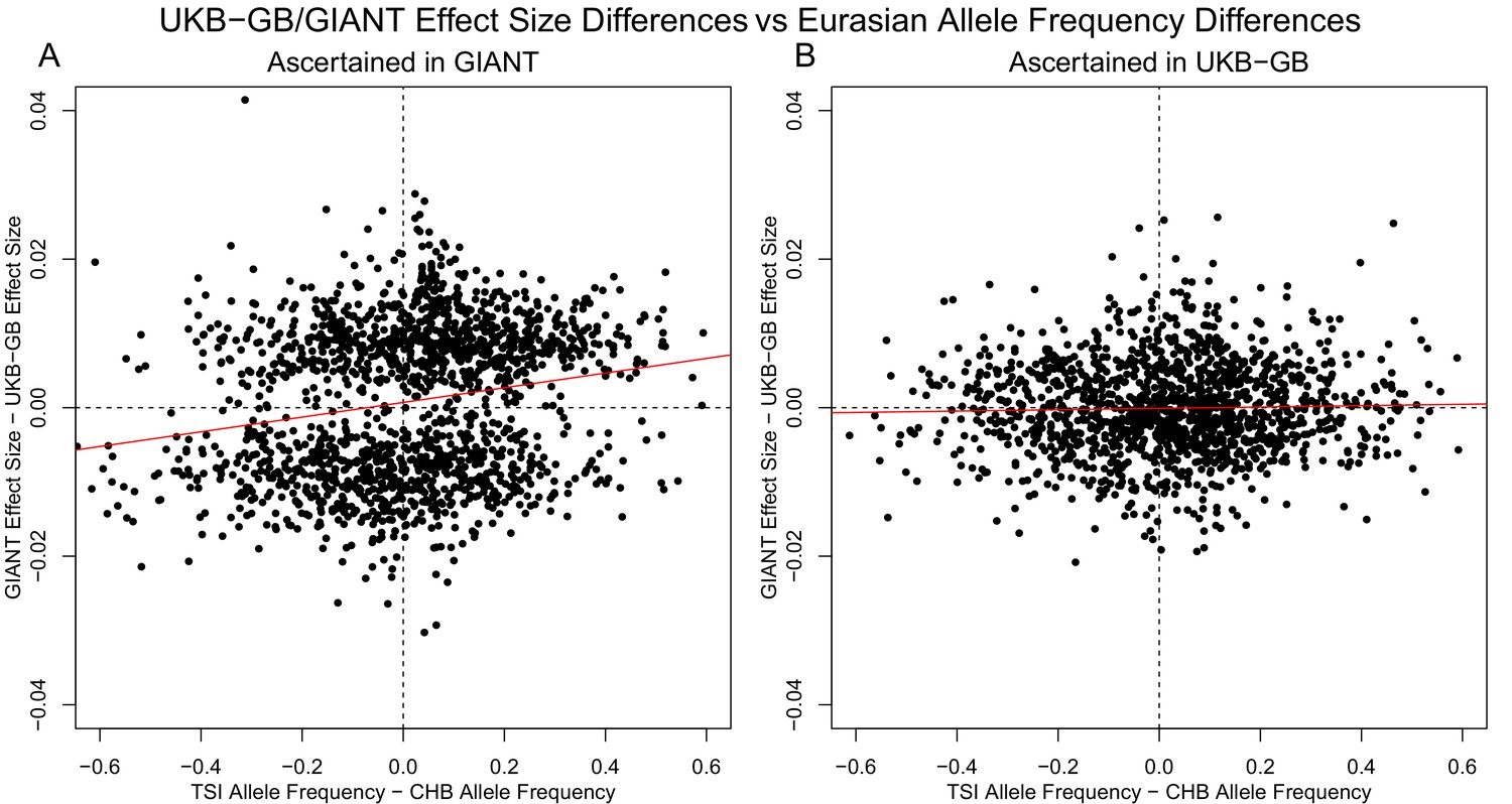
Similar patterns are seen for a TSI-CHB frequency contrast, suggesting the longitudinal patterns seen with GIANT data were also a result of stratification.
(A) SNPs are ascertained using GIANT, and the difference in effect sizes between GIANT and UKB-GB is plotted against the difference in frequency between the TSI and CHB 1000 Genomes population samples. These variables exhibit a highly significant correlation (, ). (B) SNPs are ascertained using UKB-GB, and the difference in effect sizes between GIANT and UKB-GB is again plotted against the difference in frequency between the TSI and CHB 1000 Genomes population samples. In this case, there is no significant correlation (, ).
Figure 3—figure supplement 2
The strength of the correlation between effect size difference and frequency difference is much reduced when ascertained using UKB-GB, suggesting a significant effect of ascertainment bias.
Each panel in this figure shows the same comparisons as Figure 3, except that SNPs have been ascertained with UKB-GB p-values, rather than those of GIANT or R15-sibs. Note that in both cases, the correlation between the difference in effect sizes and the GBR-TSI allele frequency difference is substantially reduced in both cases.
Figure 4 with 3 supplements
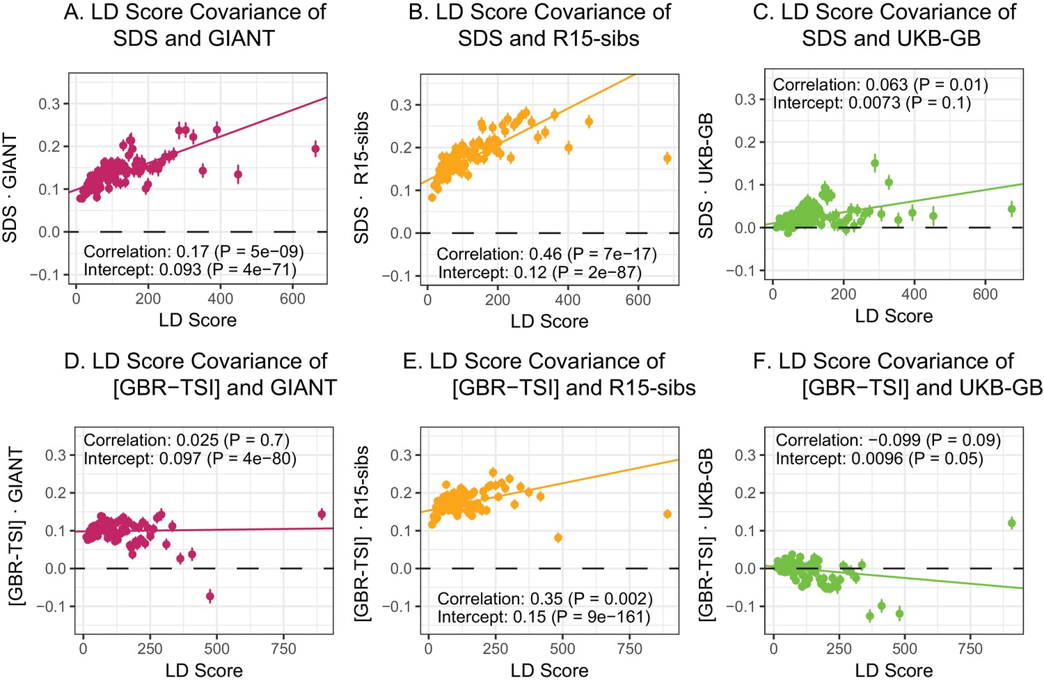
LD Score regression analyses.
(A), (B), and (C) LD Score covariance analysis of SDS with GIANT, R15-sibs, and UKB-GB, respectively. The x-axis of each plot shows LD Score, and the y-axis shows the average value of the product of effect size on height and SDS, for all SNPs in a bin. Genetic correlation estimates are a function of slope, reference LD Scores, and the sample size Bulik-Sullivan et al. (2015a). Both the slope and intercept are substantially attenuated in UKB-GB. (D), (E) and (F) Genetic covariance between GBR-TSI frequency differences vs. GIANT, R15-sibs, and UKB-GB. GIANT and R15-sibs show highly significant nonzero intercepts, consistent with a signal of population structure in both datasets, while UKB-GB does not. In addition, R15-sibs shows a significant slope with LD Score.
Figure 4—figure supplement 1
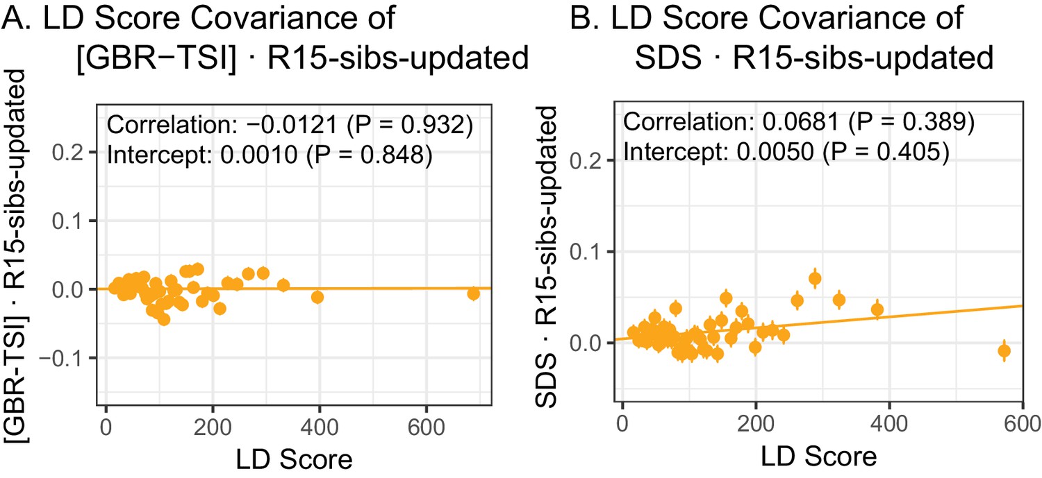
The R15-sibs-updated dataset shows no evidence of LD Score regression slope with [GBR-TSI] or with SDS.
(A) The ‘genetic correlation’ estimates of the difference in allele frequency between GBR and TSI from 1000 Genomes versus the R15-sibs-updated dataset. (B) The ‘genetic correlation’ estimates of SDS versus the R15-sibs-updated dataset.
Figure 4—figure supplement 2
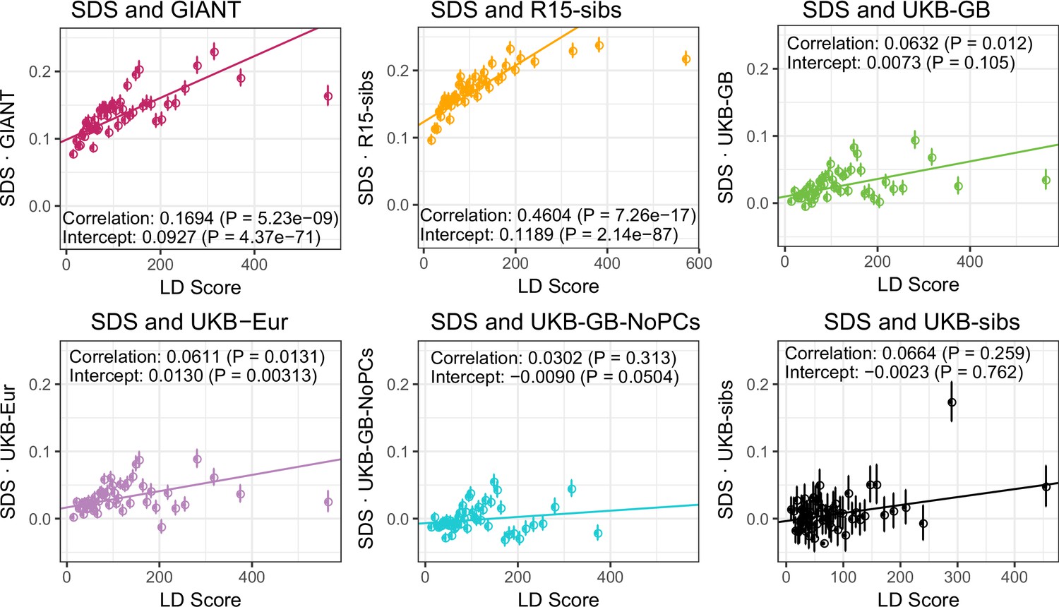
UK Biobank datasets show little evidence of bivariate LD Score regression slope when analyzed together with SDS.
Bivariate LD Score analyses of SDS with each of the height datasets.
Figure 4—figure supplement 3
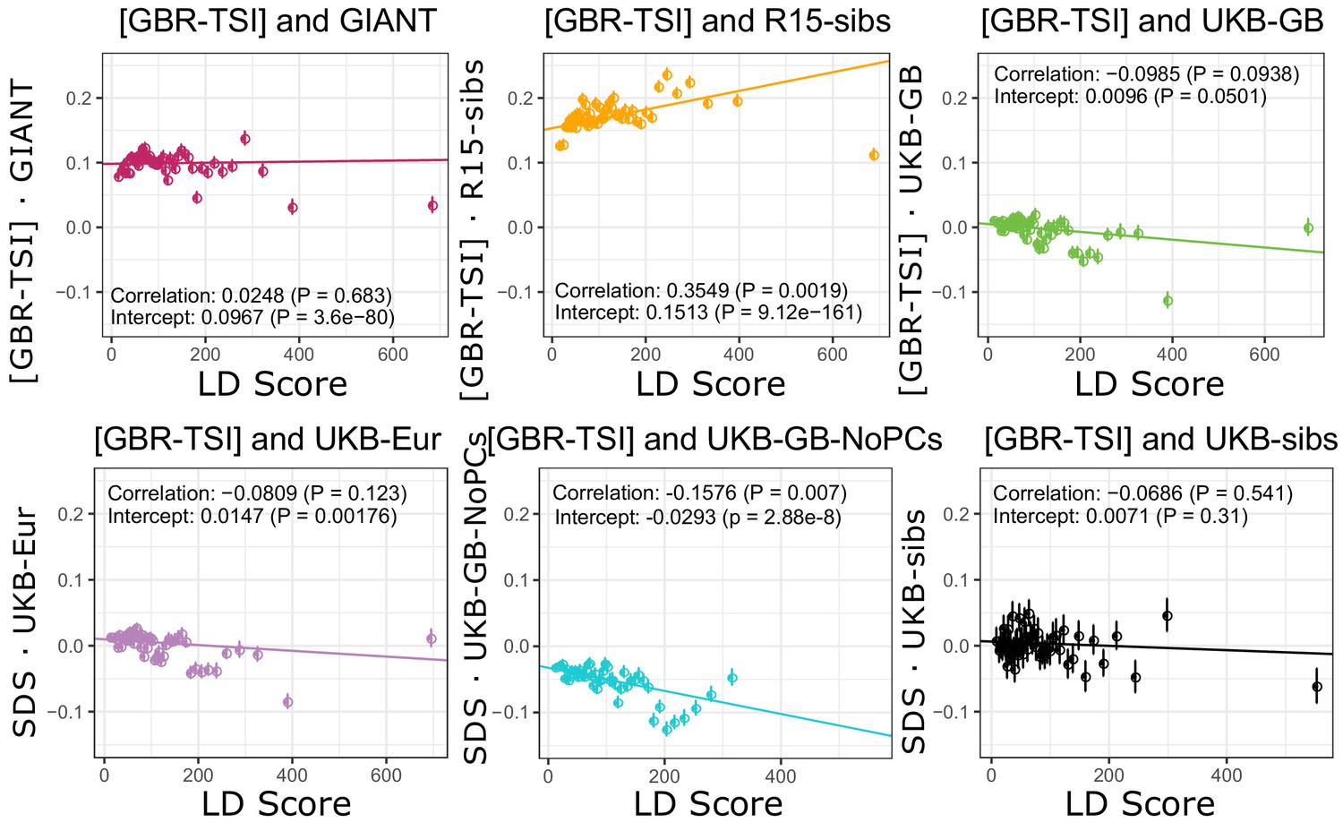
Similarly, no dataset has a significant positive slope for [GBR-TSI].
GIANT and R15-sibs show highly significant intercepts. The ‘genetic correlation’ estimates of the difference in allele frequency between GBR and TSI from 1000 Genomes versus each of the height traits under study.
Figure 5 with 1 supplement
Population allele frequencies show genetic correlation with European height GWAS.
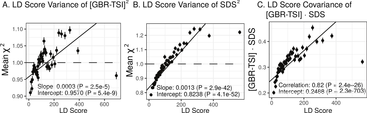
(A), (B) and (C) Magnitude of squared GBR-TSI allele frequency differences, squared SDS effect sizes, and the product of allele frequency and SDS increase with LD Score. Both SDS and GBR-TSI frequency difference are standardized and normalized within 1% minor allele frequency bins..
Figure 5—figure supplement 1
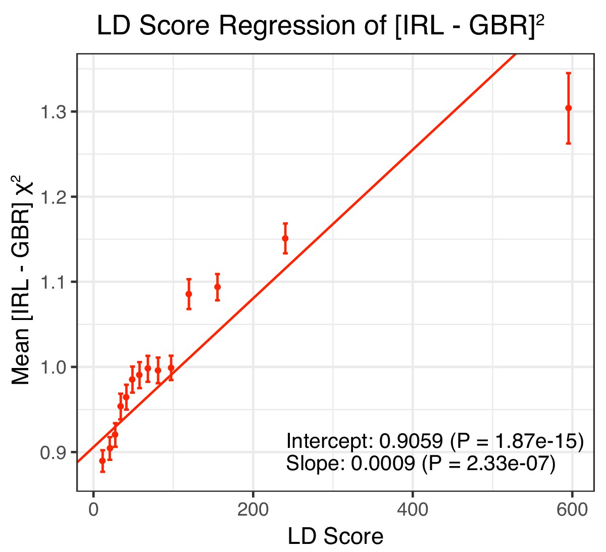
LD Score regression results for the difference in allele frequency between individuals who identified as Irish and those who identified as White British in the UK Biobank (related individuals removed).
https://doi.org/10.7554/eLife.39725.016
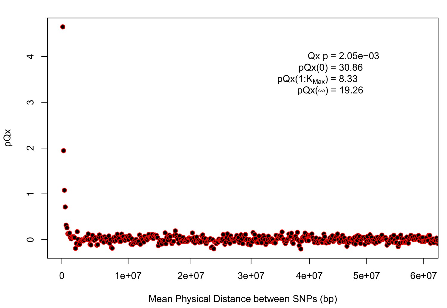
Appendix 1—figure 1
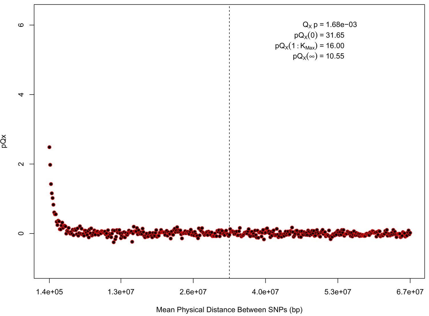
statistics for for the 20 k dataset.
The x axis gives the average physical distance between all pairs of SNPs contributing to a given statistic. The uptick in on the left side of the plot (i.e. small values of ) indicates that SNPs which are physically close to one another and have the same sign in their effect on height covary across population disproportionately as compared to more distant pairs of SNPs. Note that the number of pairs of SNPs contributing to a given decreases as increases, as smaller chromosomes have fewer pairs at larger distances than they do at shorter distances. This leads to a decrease in the variance of under the null as increases. However, this decline in variance is not responsible for the decay in signal as increases, as remains approximately constant until well past the dashed vertical line, which indicates the distance between between the ends of chromosome 21 (the shortest chromosome, and therefore the first to drop out of the calculation).
Appendix 1—figure 2
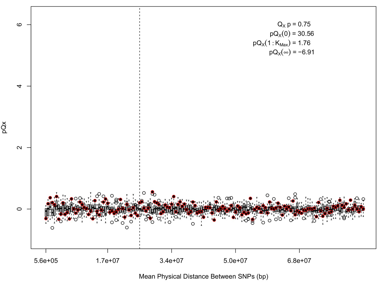
statistics for for the 5 k dataset.
The x axis gives the average physical distance between all pairs of SNPs contributing to a given statistic. The boxplots give an empirical null distribution of statistics derived from permuting the signs of all effect sizes independently (this empirical null was omitted from Appendix 1—figure 1 due to computational expense). In this case, SNPs that are physically close to one another do not contribute disproportionately to the signal.
Appendix 1—figure 3
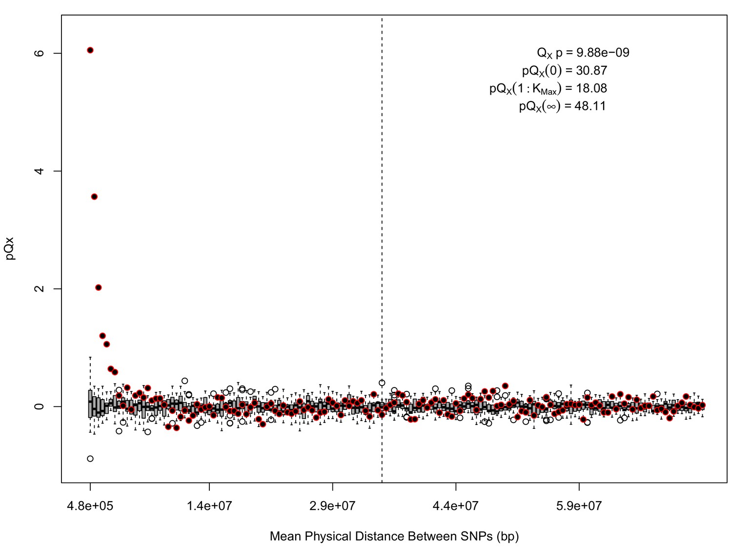
statistics for for the HapMap5k dataset.
The x axis gives the average physical distance between all pairs of SNPs contributing to a given statistic. The boxplots give an empirical null distribution of statistics derived from permuting the signs of all effect sizes independently (this empirical null was omitted from Appendix 1—figure 1 due to computational expense). The uptick in signal from pairs of SNPs physically nearby to one another is present in this dataset, again suggesting a role for physical linkage in contributing to the signal. However, note that in contrast to the 20 k and 5 k ascertainments, the HapMap5k ascertainment also has a large amount of signal from , which cannot be explained by linkage.
Appendix 1—figure 4
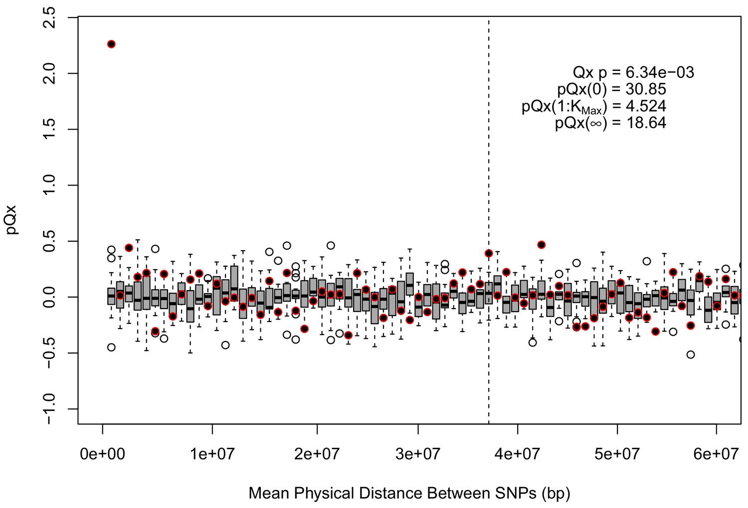
statistics for the R15-sibs-updated-3.5k ascertainment.
Similar to the expanded UKB-GB ascertainments, the elevated signal from covariance among SNPs in adjacent bins suggests that the independence assumption of the neutral model is being violated.
Appendix 1—figure 5
statistics for the R15-sibs-updated-22k.
Similar to Appendix 1—figure 4, the elevated signal from covariance among SNPs in adjacent or nearby bins suggests that the independence assumption of the neutral model is being violated. Similar to Appendix 1—figure 1, we omitted the sign flipping null due to computational expense.
Appendix 1—figure 6
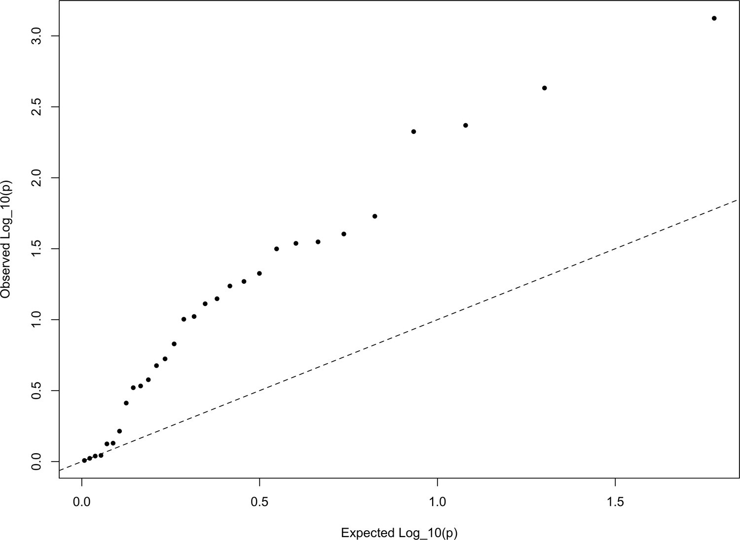
The QQ plot of P values for the statistics calculated a within-Europe sample using the HapMap5k ascertainment.
The systematic inflation of indicates a non-specific rejection of neutrality: polygenic scores are more variable in all directions than expected under the null model. This pattern is not expected under adaptive divergence of labeled populations.
Appendix 2—figure 1
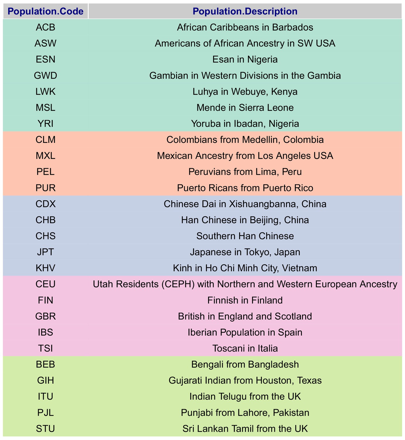
Present-day populations from 1000 Genomes Project Phase 3 used to build population-level polygenic scores, colored by their respective super-population code.
https://doi.org/10.7554/eLife.39725.026
Appendix 2—figure 2
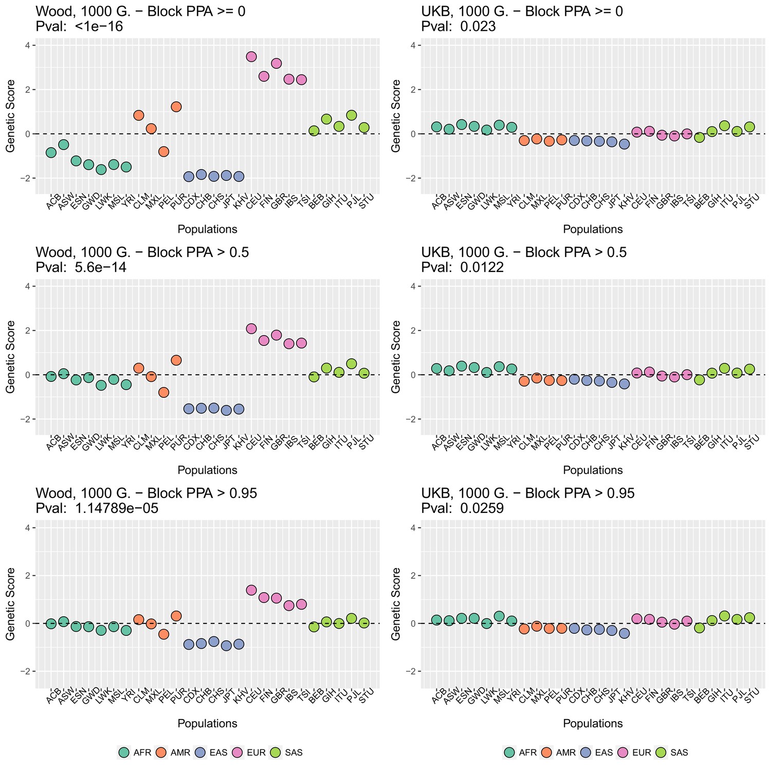
Genetic scores in present-day populations, colored by their super-population code, and created using different block-PPA thresholds.
Left column: Wood et al. (2014) GWAS. Right column: Neale lab UK Biobank GWAS.
Appendix 2—figure 3

Distribution of the absolute value of effect sizes (y-axis) plotted as a function of the difference in frequency of the trait-increasing allele between CEU and CHB (x-axis), for candidate SNPs used to build genetic scores.
Top left: trait-associated SNPs from Wood et al., with effect sizes from the same GWAS. Top right: trait-associated SNPs from the Neale lab GWAS, with effect sizes from the same GWAS. Bottom left: trait-associated SNPs from Wood et al., but with their corresponding effect sizes from the Neale lab GWAS. Bottom right: trait-associated SNPs from the Neale lab GWAS, but with their corresponding effect sizes from Wood et al. Contour colors denote the density of SNPs in different regions of each plot.
Appendix 2—figure 4
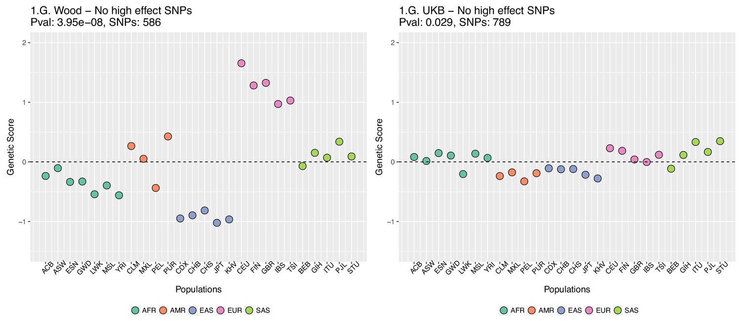
Genetic scores for present-day populations, after excluding 6 high-effect SNPs from UKB, colored by super-population code.
Left: Wood et al. GWAS. Right: Neale lab UK Biobank GWAS.
Appendix 2—figure 5
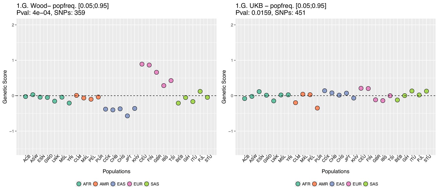
Genetic scores computed only with SNPs that have minor allele frequencies larger than 0.05 in all populations.
Left: Wood et al. GWAS. Right: Neale lab UK Biobank GWAS.
Appendix 2—figure 6

Genetic scores computed using the UK Biobank data, after removing SNPs with absolute effect sizes smaller than or equal to 0.05 in Wood et al.
https://doi.org/10.7554/eLife.39725.031
Appendix 2—figure 7

Genetic scores computed using the UK Biobank data, after removing SNPs with absolute effect sizes smaller than or equal to 0.01 in Wood et al.
https://doi.org/10.7554/eLife.39725.032
Appendix 3—figure 1
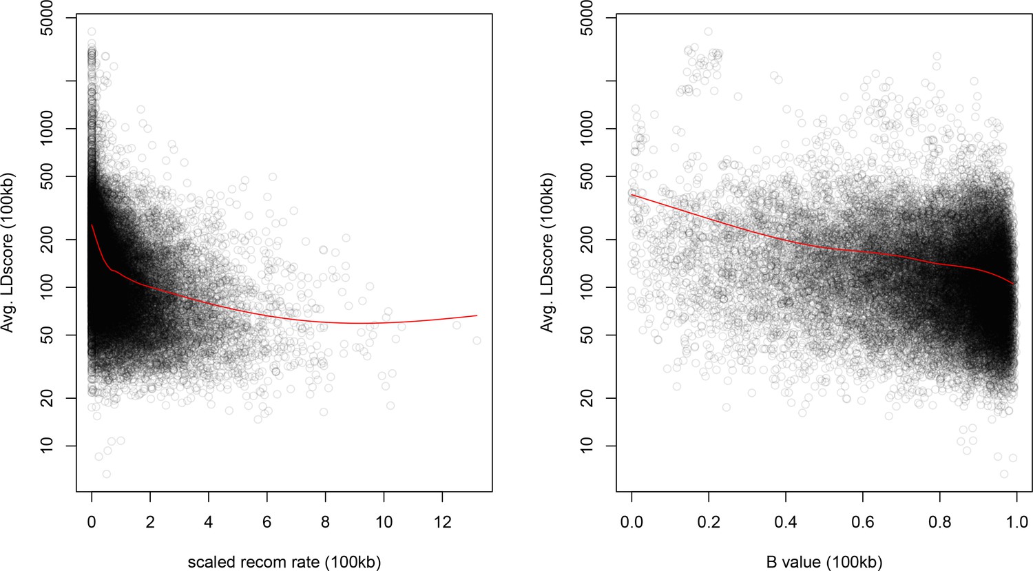
Windows with lower recombination rates and B values have higher LD Scores.
The autosome is divided into 100 kb windows and the average LD Score, B-value, and standardized recombination rate is calculated in each bin. The red lines are a lowess fit as a guide to the eye.
Appendix 3—figure 2
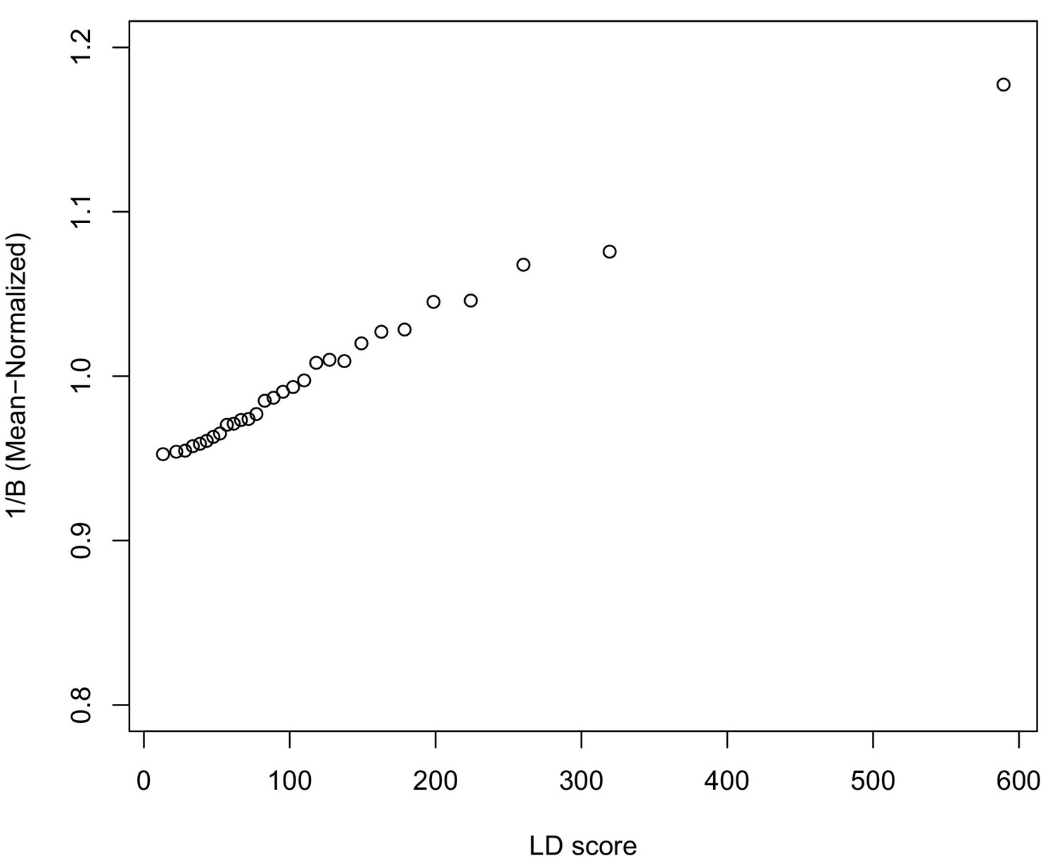
A plot across 30 quantiles of genome-wide LD Score of our simple BGS model of differentiation, parameterized by McVicker’s B (Equation A11).
https://doi.org/10.7554/eLife.39725.035
Appendix 3—figure 3
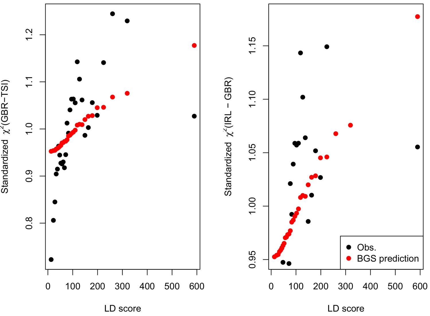
A plot across 30 quantiles of LD Score a standardized (Equation A11) of allele frequency differentiation (black dots) and that expected under our simple BGS model parameterized by McVicker’s B (red dots, Equation A11, standardized by its genome-wide mean).
Note that the red dots are the same values in both panels, and match those given in Figure 2.
Appendix 4—figure 1
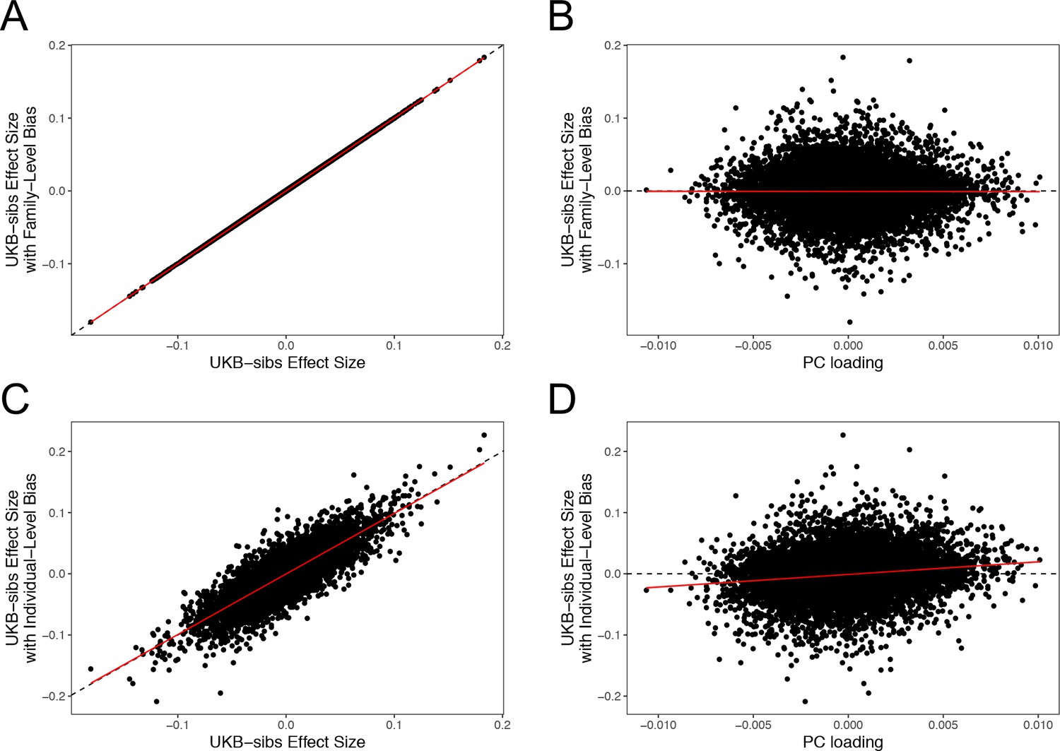
QFAM effect size estimates, under two population stratification scenarios.
Top Row: Height values made biased along PC5-axis, proportional to the mean PC5 scores within family. (A) The x- and y-axes show effect size estimates without and with the added bias, respectively. (B) The x-axis shows the SNP loadings on PC5. Bottom Row: Height values made biased along PC5-axis, proportional to individuals’ PC5 scores. (C) The same plot as panel (A), but with individual-level bias. (D) The same plot as panel (B), but with individual-level bias. All results are shown for 11,611 SNPs on chromosome one for which PC loadings where provided by the UK Biobank.
Tables
Table 1
Studies reporting signals of height adaptation in Europeans.
Prior to the UK Biobank dataset, studies consistently found evidence for polygenic adaptation of height. Notes: Most of the papers marked as having ‘strong’ signals report p-values , and sometimes . In the present paper, the UK Biobank analyses generally yield p-values .
| GWAS | Approach | Signal | Reference |
|---|---|---|---|
| GIANT 2010 | European frequency cline of top SNPs | strong | Turchin et al., 2012 |
| validation: Framingham sibs | |||
| GIANT 2010 | Polygenic measures of pop. frequency differences | strong | Berg and Coop, 2014 |
| GIANT | Polygenic measures of pop. frequency differences | strong | Berg et al., 2017 |
| strong | Racimo et al., 2018 | ||
| strong | Guo et al., 2018 | ||
| Polygenic diffs between ancient and modern populations | strong | Mathieson et al., 2015 | |
| GIANT | Heterogeneity of polygenic scores among populations | strong | Robinson et al., 2015 |
| validation: R15-sibs | |||
| Sardinia cohort | Low polygenic height scores in Sardinians. Effect estimates from Sardinian cohort at GIANT hit SNPs | strong | Zoledziewska et al., 2015 |
| GIANT and R15-sibs | Singleton density (SDS) in UK sample vs GWAS | strong | Field et al., 2016 |
| Also: LD Score regression (SDS vs GWAS) | strong | ||
| UK Biobank | Population frequency differences | weak or absent | This paper* |
| Singleton density (SDS) in UK sample | weak or absent | This paper* | |
| LD Score regression (SDS vs GWAS) | weak | This paper* |
-
*See also results from Sohail et al., 2019.
Table 2
Pairwise genetic correlations between GWAS datasets.
Genetic correlation estimates (lower triangle) and their standard errors (upper triangle) between each of the height datasets, estimated using LD Score regression (Bulik-Sullivan et al., 2015a). All trait pairs show a strong genetic correlation, as expected for different studies of the same trait.
| Giant | R15-sibs | UKB-Eur | UKB-GB-NoPCs | Ukb-gb | UKB-sibs | |
|---|---|---|---|---|---|---|
| GIANT | (0.04) | (0.01) | (0.01) | (0.01) | (0.05) | |
| R15-sibs | 0.98 | (0.04) | (0.04) | (0.05) | (0.08) | |
| UKB-Eur | 1.03 | 0.87 | (0.004) | (0.004) | (0.05) | |
| UKB-GB-NoPCs | 1.01 | 0.82 | 1.00 | (0.002) | (0.05) | |
| UKB-GB | 1.03 | 0.89 | 1.02 | 1.00 | (0.05) | |
| UKB-sibs | 1.02 | 0.93 | 1.06 | 1.02 | 1.06 |
Additional files
-
Transparent reporting form
- https://doi.org/10.7554/eLife.39725.017
Download links
A two-part list of links to download the article, or parts of the article, in various formats.
Downloads (link to download the article as PDF)
Open citations (links to open the citations from this article in various online reference manager services)
Cite this article (links to download the citations from this article in formats compatible with various reference manager tools)
Reduced signal for polygenic adaptation of height in UK Biobank
eLife 8:e39725.
https://doi.org/10.7554/eLife.39725


