Extrinsic and intrinsic dynamics in movement intermittency
- Newcastle University, United Kingdom
Figures
Figure 1 with 3 supplements
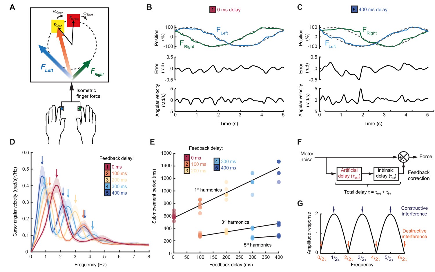
Movement intermittency during visuomotor tracking depends on feedback delays.
(A) Schematic of human tracking task. Bimanual isometric finger forces controlled 2D cursor position to track slow, circular target motion. Kinematic analyses used the angular velocity of the cursor subtended at the screen center during the middle of each trial. (B) Example force (top), angular error (middle) and cursor angular velocity (bottom) traces during target tracking with no feedback delay. Submovements are evident as intermittent fluctuations in angular velocity. (C) Example movement traces with 400 ms feedback delay. (D) Power spectra of cursor angular velocity with different feedback delays between 0 and 400 ms. Analysis based on a 10 s window beginning 5 s after trial start. Average of 8 subjects, shading indicates standard error of mean (s.e.m.). See also Figure 1—figure supplement 2. (E) Submovement periods (reciprocal of the peak frequency for each harmonic) for all subjects with different feedback delays. Lines indicate linear regression over all subjects. See Table 1 for summary of individual subject regression analysis. (F) Schematic of a simple delayed feedback controller. (G) Amplitude response of the system shown in (F), known as a comb filter.
-
Figure 1—source data 1
Subject information, time periods of submovement peaks and associated regression analysis.
- https://doi.org/10.7554/eLife.40145.006
Figure 1—figure supplement 1
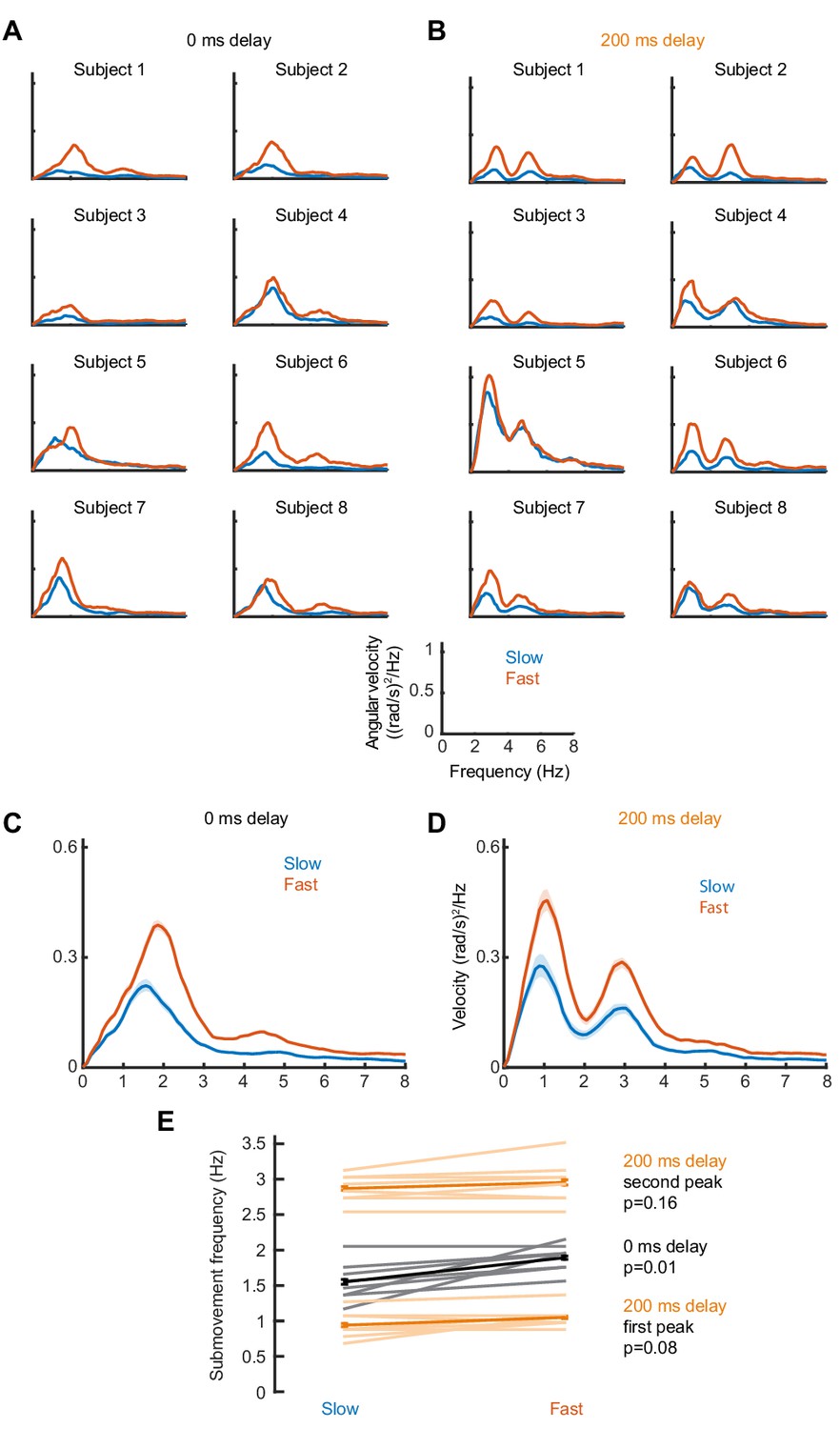
Effect of target speed on movement intermittency.
(A) Power spectra of cursor angular velocity for individual subjects with slow (0.1 cycles/s) or fast (0.2 cycles/s) target rotation, and no feedback delay. (B) Power spectra of cursor angular velocity with slow or fast target rotation, and 200 ms feedback delay. (C,D) Average power, showing mean ± s.e.m. for eight subjects. (E) Average ± s.e.m. frequencies of peak cursor velocity in each condition. P values calculated using a paired t-test.
Figure 1—figure supplement 2

Individual subject power spectra of cursor velocity with different feedback delays.
Power spectra of cursor angular velocity for individual subjects with 0–400 ms feedback delay. The average over subjects is shown in Figure 1D.
Figure 1—figure supplement 3
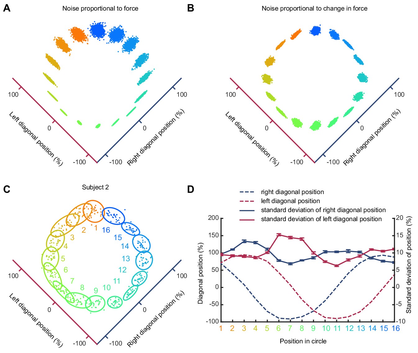
Trajectory variability depends on change in isometric force.
(A) Simulated pattern of trial-to-trial variability if motor noise is proportional to absolute force. (B) Simulated pattern of trial-to-trial variability if motor noise is proportional to derivative of force. (C) Variability of a typical subject during counter clockwise tracking. 2D cursor position over multiple trials and associated covariance ellipses are shown for 16 target positions. (D) Average and s.e.m. of standard deviation of force along each finger axis for the 16 target positions. Note that variability is maximal at times of maximal change in associated finger force (dashed lines).
Figure 2 with 3 supplements
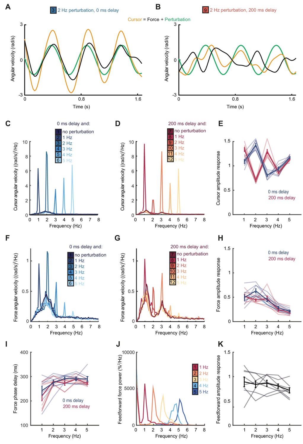
Frequency responses and phase delays to artificial motor errors.
(A) Example force (black) and cursor (yellow) angular velocity traces in the presence of a 2 Hz perturbation (green) when no feedback delay was added. The force response and perturbation sum to produce large fluctuations in cursor velocity. (B) Comparable data with a feedback delay of 200 ms. In this condition, force responses cancel the perturbation leading to an attenuation of intermittency. (C) Power spectra of cursor angular velocity with 1–5 Hz perturbations and no feedback delay. Analysis based on 10 s windows beginning 5 s after trial start. Average of 8 subjects. See also Figure 2—figure supplement 1. (D) Power spectra of cursor angular velocity with 1–5 Hz perturbations and 200 ms feedback delay. (E) Cursor amplitude response to 1–5 Hz perturbations with no feedback delay (blue) and 200 ms feedback delay (red) for individual subjects. Also shown is the average ± s.e.m. of 8 subjects. (F) Power spectra of force angular velocity with 1–5 Hz perturbations and no feedback delay. See also Figure 2—figure supplement 2. (G) Power spectra of force angular velocity with 1–5 Hz perturbations and 200 ms feedback delay. (H) Force amplitude response to 1–5 Hz perturbations with no feedback delay (blue) and 200 ms feedback delay (red). Also shown is average ± s.e.m. of 8 subjects. (I) Intrinsic phase delay of force response to 1–5 Hz perturbations with no feedback delay (blue) and 200 ms feedback delay (red). Also shown is average ± s.e.m. of 8 subjects. (J) Power spectrum of finger forces generated in the feedforward task with auditory cues at 15 Hz. Average of 8 subjects. See also Figure 2—figure supplement 3. (K) Force amplitude response to auditory cues in the feedforward task. Also shown is average ± s.e.m. of 8 subjects. All analyses based on a 10 s windows beginning 5 s after trial start.
-
Figure 2—source data 1
Subject information, perturbation responses and feedforward amplitude responses.
Data for individual subjects in Experiment 2 (summarized in Figure 2C–I) and Experiment 3 (summarized in Figure 2K).
- https://doi.org/10.7554/eLife.40145.012
Figure 2—figure supplement 1
Individual subject power spectra of cursor velocity with perturbations.
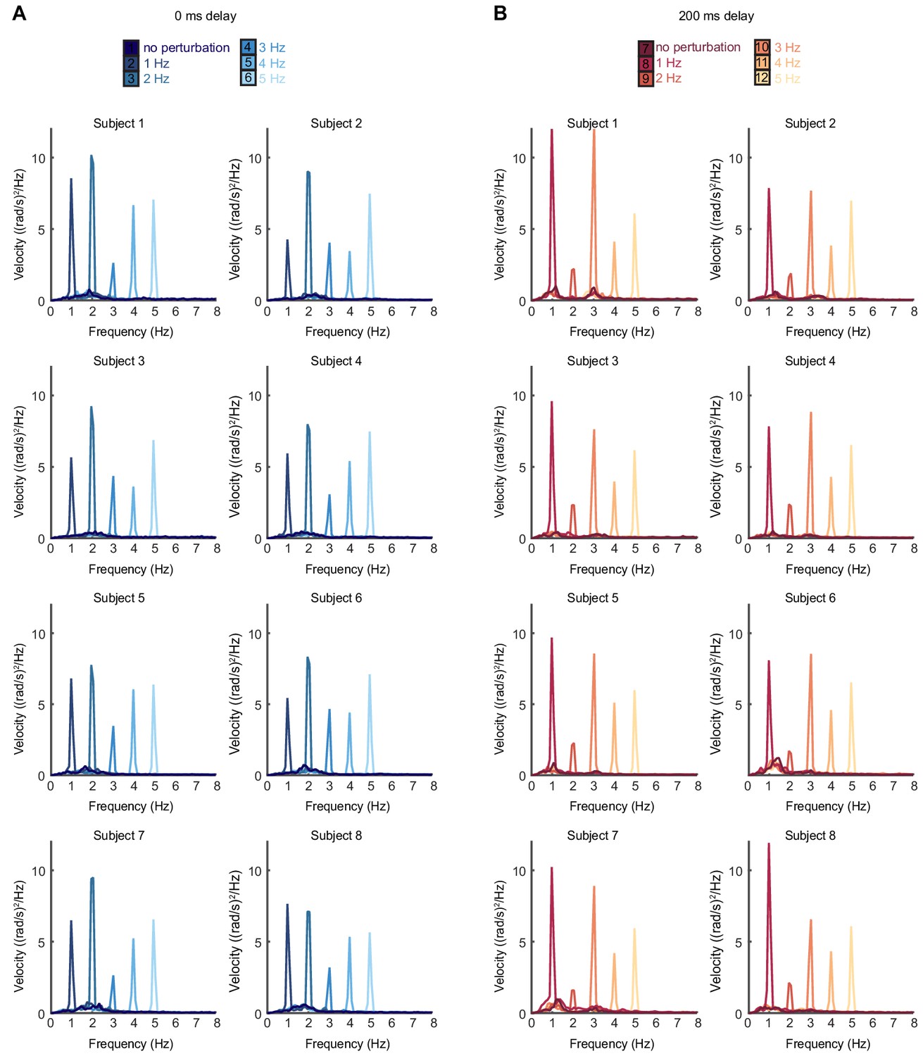
(A) Power spectra of cursor angular velocity for individual subjects with 1–5 Hz perturbations and no feedback delay. The average over subjects is shown in Figure 2C. (B) Power spectra of cursor angular velocity for individual subjects with 1–5 Hz perturbations and 200 ms feedback delay. The average over subjects is shown in Figure 2D.
Figure 2—figure supplement 2
Individual subject power spectra of force velocity with perturbations.
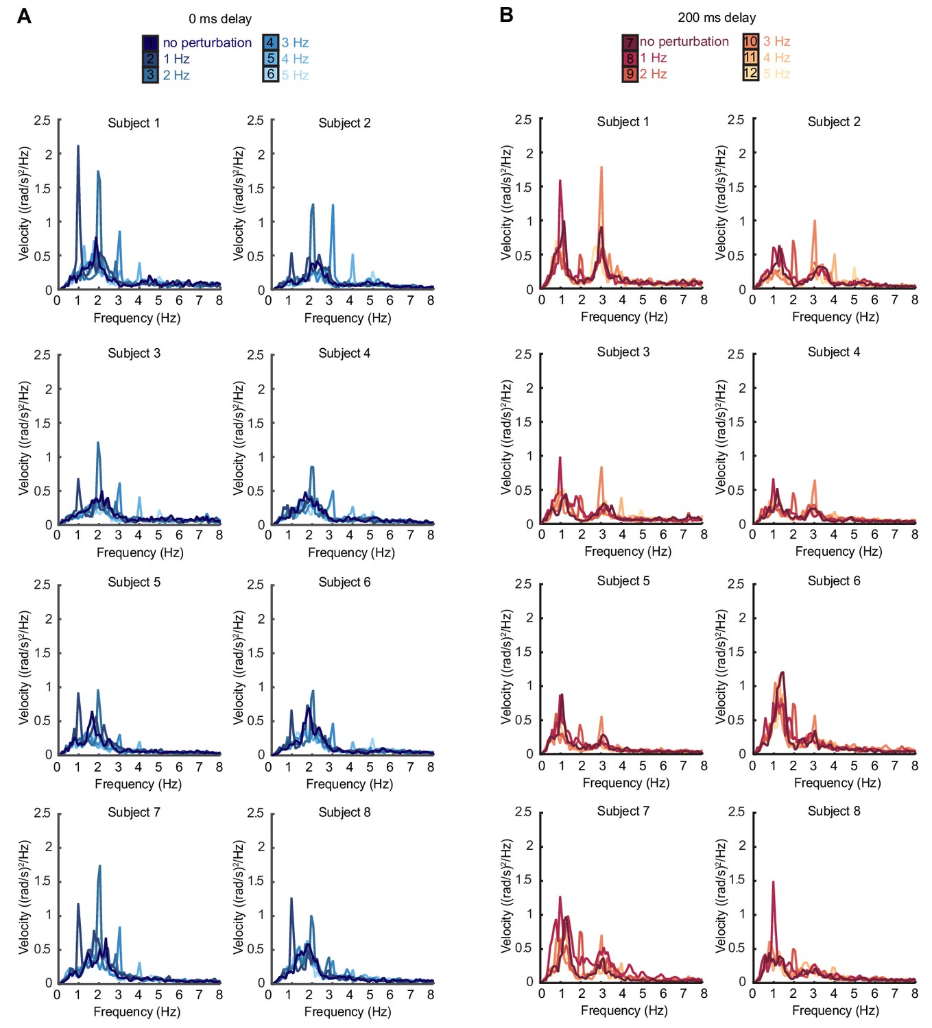
(A) Power spectra of force angular velocity for individual subjects with 1–5 Hz perturbations and no feedback delay. The average over subjects is shown in Figure 2F. (B) Power spectra of force angular velocity for individual subjects with 1–5 Hz perturbations and 200 ms feedback delay. The average over subjects is shown in Figure 2G.
Figure 2—figure supplement 3
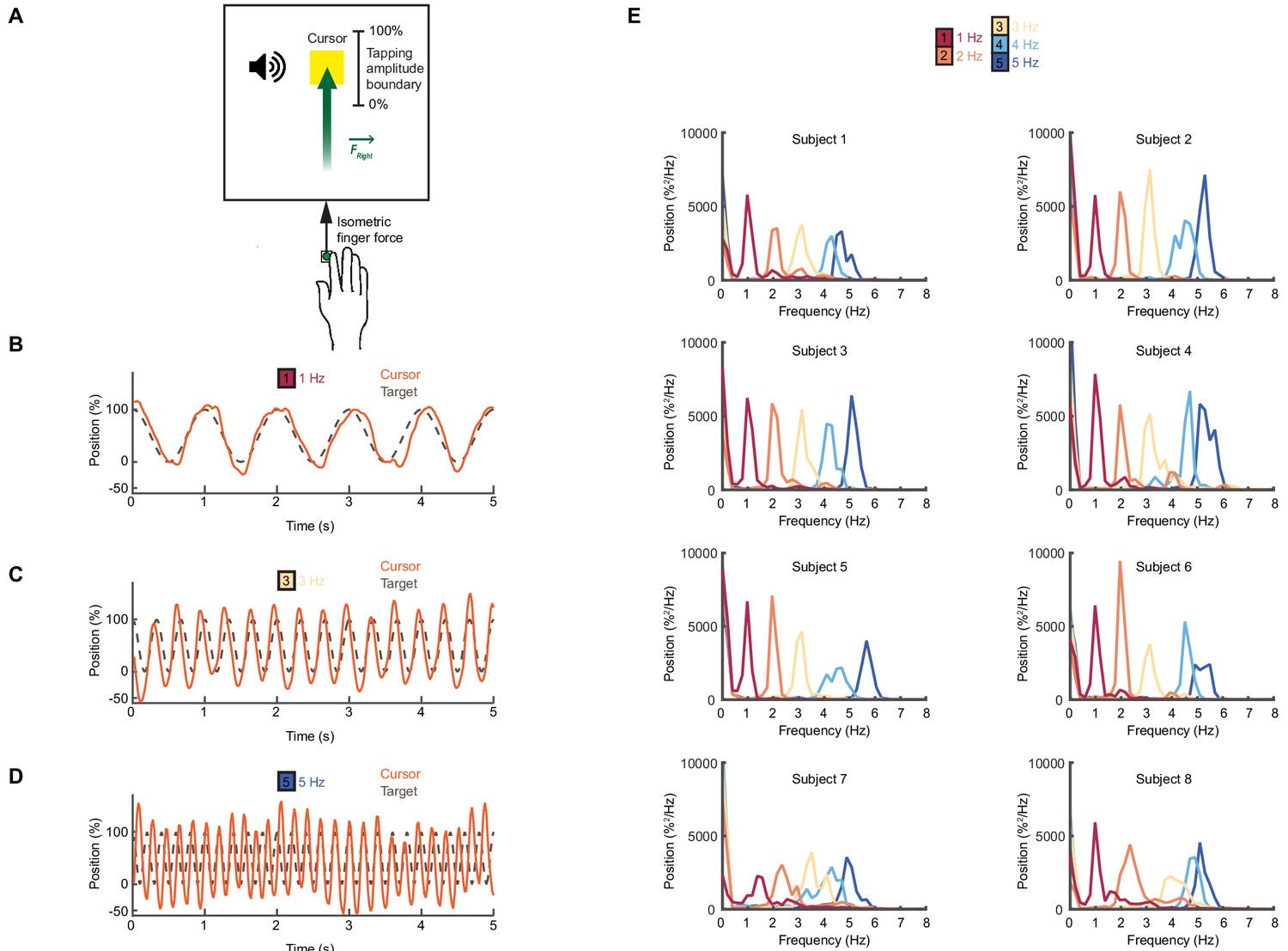
Feedforward task.
(A) Schematic of the feedforward isometric task. Subjects generated sinusoidal forces within a set range, at a frequency indicated by an auditory cue. (B–D) Performance of an example subject for frequencies between 1–5 Hz. (E) Power spectrum of force for individual subjects. The average over all subjects is shown in Figure 2J.
Figure 3
State estimation with a Kalman filter.
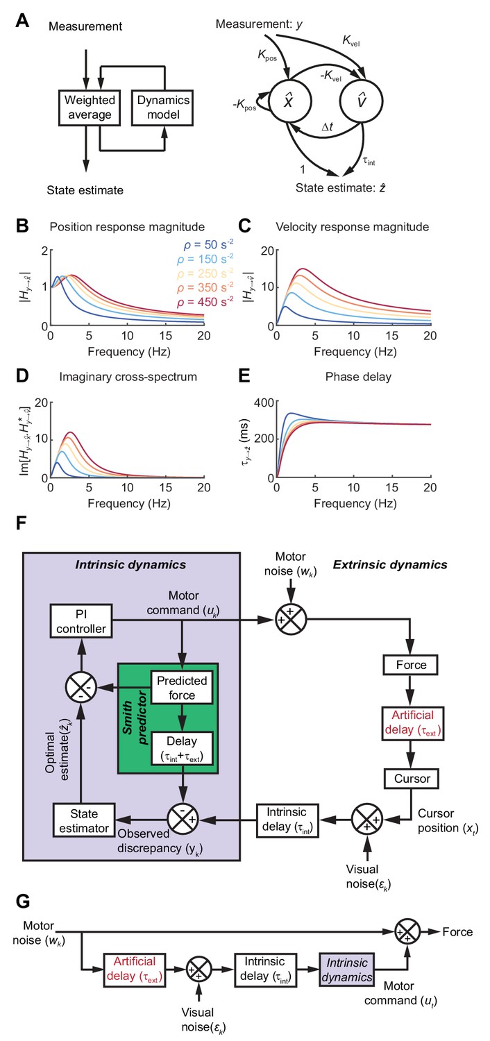
(A) Left: Schematic of a Kalman filter. Noisy measurements are combined with an internal model of the external dynamics to update an optimal estimate of current state. Right: A dynamical system for optimal estimation of position, based on an internal model of position and velocity. (B, C) Magnitude response of transfer function from measurement to position and velocity estimates, respectively, for a Kalman filter with different ratios of process to measurement noise (). (D) Imaginary component of cross-spectrum between position and velocity transfer functions. (E) Phase delay of optimal estimate of position based on delayed measurement of position. (F) Schematic of optimal feedback controller model incorporating state estimation and a Smith Predictor architecture to accommodate feedback delays. (G) Simplified rearrangement of (F), showing the feedforward relationship between motor noise and force output. This rearrangement is possible because the Smith Predictor prevents motor corrections reverberating multiple times around the feedback loop.
Figure 4
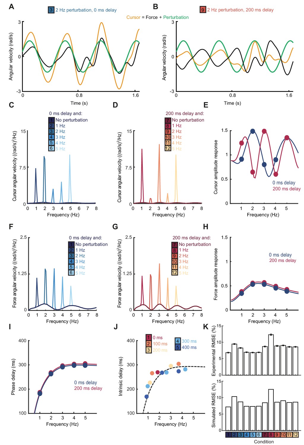
Smith Predictor model with optimal state estimation reproduces human behavioral data.
(A) Simulated tracking performance of the model with a 2 Hz sinusoidal perturbation and no feedback delay. (B) Simulated tracking performance of the model with a 2 Hz sinusoidal perturbation and 200 ms feedback delay. (C) Power spectrum of simulated cursor velocity with 1–5 Hz perturbations and no feedback delay. (D) Power spectrum of simulated cursor velocity with 1–5 Hz perturbations and 200 ms feedback delay. (E) Simulated cursor amplitude response to 1–5 Hz perturbations with no feedback delay (blue) and 200 ms feedback delay (red). (F) Power spectrum of simulated force velocity with 1–5 Hz perturbations and no feedback delay. (G) Power spectrum of simulated force velocity with 1–5 Hz perturbations and 200 ms feedback delay. (H) Simulated force amplitude response to 1–5 Hz perturbations with no feedback delay (blue) and 200 ms feedback delay (red). (I) Simulated intrinsic phase delay of force responses to 1–5 Hz perturbations with no feedback delay (blue) and 200 ms feedback delay (red). (J) Intrinsic delay times corresponding to all submovement peaks/harmonics in Figure 1D, plotted against the frequency of the peak. Dashed line indicates phase delay of the simulated optimal controller (K) Top: Positional inaccuracy of human tracking for all conditions quantified as root mean squared error (RMSE). Average ± s.e.m. of 8 subjects. Bottom: RMSE of simulated tracking for all conditions.
Figure 5
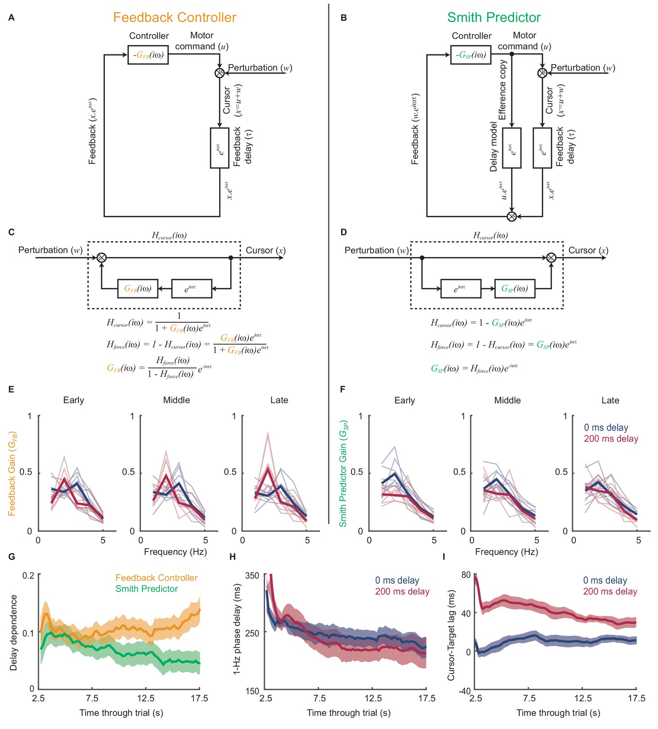
Emergence of predictive control strategies within individual trials.
(A) Schematic of a simple feedback controller with intrinsic gain, and time delay, . (B) A Smith Predictor with intrinsic gain, , time delay and calibrated internal feedback loop. (C,D) Rearrangements of the two model architectures to allow derivation of the cursor response function, , and force amplitude response, . Note that both act as ‘comb filters’ and exhibit delay-dependent submovement peaks. However the architectures predict different relationships between intrinsic gain and force amplitude response. (E) Feedback gains inferred from experimental data assuming the simple feedback controller architecture, for 5 s windows early, middle and late in each trial. Thick line shows average over 8 subjects. Note that feedback gains for different delay conditions become less similar as the trial progresses. (F) Feedback gains inferred from experimental data assuming the Smith Predictor architecture. Feedback gains for different delay conditions become more similar as trial progresses. (G) Delay-dependence of feedback gain (mean-squared difference between delay conditions) inferred from the two architectures. The analysis used a 5 s sliding window through the entire trial. Shading indicates s.e.m. over 8 subjects. (H) Phase delay of feedback gain at 1 Hz inferred from Smith Predictor architecture through trials with 0 and 200 ms delay. (I) Average time lag between cursor and target through trials with 0 and 200 ms delay (and no spatial perturbation).
Figure 6

Movement intermittency in a non-human primate tracking task.
(A) Radial cursor position during a typical trial of the center-out isometric wrist torque task under two different feedback delay conditions. Data from Monkey U. (B) Radial cursor velocity. Arrowheads indicate time of submovements identified as positive peaks in radial cursor velocity. (C) Low-pass filtered, mean-subtracted LFPs from M1. (D) First two principal components (PCs) of the LFP. (E) The second LFP-PC overlaid on the radial cursor velocity.
Figure 7

Frequency-domain analysis reveals delay-dependent and delay-independent spectral features.
(A) Power spectrum of radial cursor speed with 0–600 ms feedback delay. Traces have been off-set for clarity. Arrows indicate expected frequencies of peaks from OFC model. Data from Monkey U. (B) Average power spectrum of M1 LFPs. (C) Average coherence spectrum between radial cursor speed and all M1 LFPs. (D) Average imaginary coherence spectrum between all pairs of M1 LFPs. (E–H) As above, but for Monkey S. (I–L) Simulated power and coherence spectra produced by the OFC model.
Figure 8 with 1 supplement
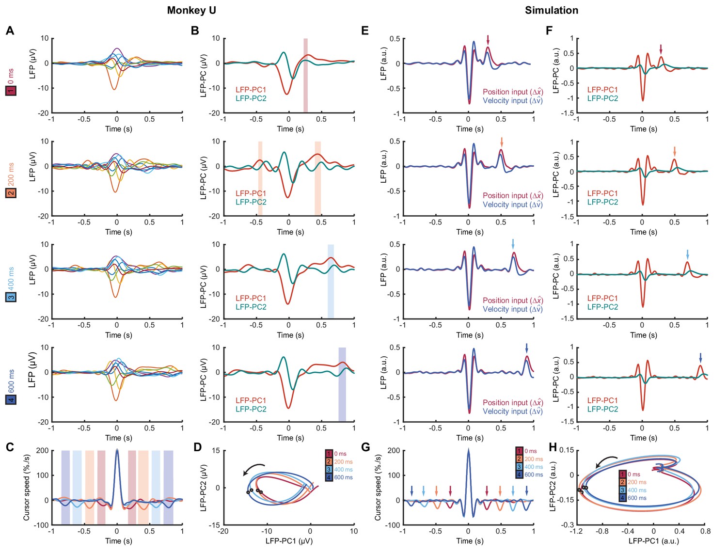
Submovement-triggered averages of M1 LFPs.
(A) Average low-pass filtered LFPs from M1, aligned to the peak speed of submovements with 0–600 ms feedback delay. Note the second feature, which follows submovements by an extrinsic, delay-dependent latency. Data from Monkey U. See also Figure 8—figure supplement 1. (B) Average of first two LFP-PCs aligned to submovements. Shading indicates significant delay-dependent peaks in PC1 (p<0.001, Kruskal-Wallis test and post-hoc signed-ranks test across delay conditions). (C) Average low-pass filtered cursor speed, aligned to submovements. Shading indicates significant (p<0.001) delay-dependent troughs. (D) Average submovement-triggered LFP-PC trajectories, plotted over 200 ms either side of the time of peak submovement speed (indicated by circles). (E–H) Simulated submovement-triggered averages produced by the OFC model.
Figure 8—figure supplement 1
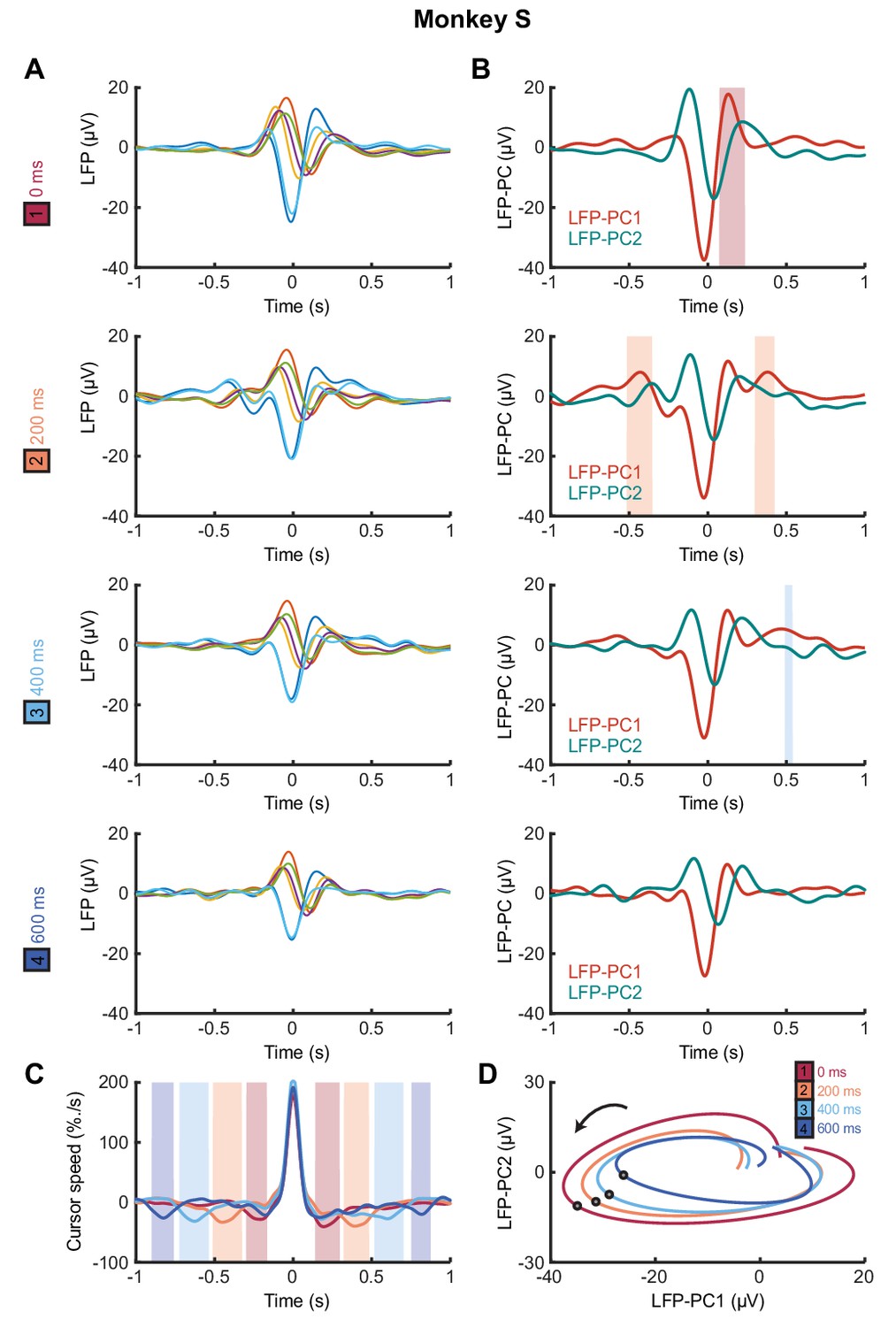
Submovement-triggered averages of M1 LFPs for Monkey S.
(A) Average low-pass filtered LFPs from M1, aligned to the peak speed of submovements with 0–600 ms feedback delay. Data from Monkey S. (B) Average of first two LFP-PCs aligned to submovements. Shading indicates significant delay-dependent peaks in PC1 (p<0.05, Kruskal-Wallis test and post-hoc signed-ranks test across delay conditions). (C) Average low-pass filtered cursor speed, aligned to submovements. Shading indicates significant (p<0.05) delay-dependent troughs. (D) Average submovement-triggered LFP-PC trajectories, plotted over 200 ms either side of the time of peak submovement speed (indicated by circles).
Figure 9
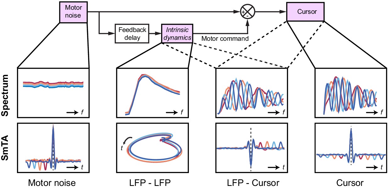
Schematic of delay-dependent and delay-independent relationships in the OFC model.
The boxes show how the various frequency-domain and submovement-triggered average (SmTA) relationships are explained by the OFC model. Top row, from left to right: Broad spectrum motor noise drives intrinsic dynamics resulting in a delay-independent LFP cross-spectral resonance. The delayed motor command is combined with the original motor noise leading to delay-dependent comb filtering, evident in LFP-Cursor coherence and Cursor power spectrum. Bottom row, from left to right: submovements can arise from a positive noise peak at time-zero, or as a correction to a preceding negative noise trough. Due to intrinsic dynamics, LFPs trace consistent cyclical trajectories locked to submovements. SmTA of LFPs contains potentials associated with noise peak/troughs after feedback delay. SmTA of cursor velocity combines noise with delayed feedback corrections to yield a central submovement flanked by symmetrical troughs.
Figure 10
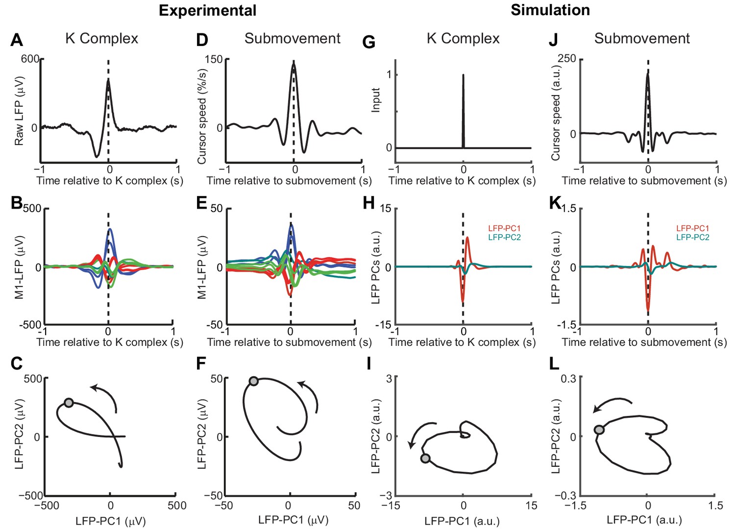
Simulated LFP dynamics during movement and sedation.
(A) K-complex events in LFP from M1 recorded under ketamine sedation. (B) Average low-pass filtered multichannel LFPs aligned to K-complex events. LFPs are color-coded according to phase relative to submovements, but exhibit a similar pattern relative to K-complexes. (C) Average LFP-PC trajectories aligned to K-complexes, plotted over 200 ms either side of the time of the K-complex (indicated by a circle), using the PC plane calculated from recordings during awake behavior. (D) Average cursor speed aligned to the peak speed of submovements. (E) Average low-pass filtered multichannel LFPs aligned to submovements. (F) Average submovement-triggered LFP-PC trajectories, plotted over 200 ms either side of the time of submovements (indicated by a circle). (G) A K-complex under sedation is simulated by an impulse excitation of the OFC model, without connection to the external world. (H) Impulse response of the simulated LFP-PCs. (I) LFP-PC trajectories associated with simulated K-complexes. (J) Simulated submovement-triggered average cursor speed from the OFC model with no feedback delay. (K) Simulated submovement-triggered average LFP-PCs. (L) Simulated submovement-triggered LFP-PC trajectories. Panels A–F reproduced from Figure 4A,C,E in Hall et al. (2014) (published under a Creative Commons CC BY 3.0 license).
Tables
Table 1
The dependency of submovement period on feedback delay.
Shown in the table are the gradients and intercepts of regression lines fitted to each harmonic group in Figure 1E. The time period of each spectral peak was regressed against feedback delay. Shown in square brackets are 95% confidence intervals of these values. Also shown is the estimated intrinsic time delay calculated using Equation (1).
| Harmonic (N) | Predicted slope = 2/N | Measured slope | Measured intercept (ms) | R2 | P | τint = Intercept*N/2 |
|---|---|---|---|---|---|---|
| 1 | 2 | 1.89 [1.69,2.09] | 589 ms [539,638] | 0.90 | <0.00001 | 294 ms [270,319] |
| 3 | 0.67 | 0.59 [0.53,0.65] | 226 ms [211,242] | 0.94 | <0.00001 | 340 ms [316,362] |
| 5 | 0.4 | 0.33 [0.22,0.45] | 146 ms [106,185] | 0.75 | <0.00001 | 364 ms [266,463] |
Additional files
-
Source code 1
MATLAB implementation of feedback controller model.
Code used to generate Figure 4.
- https://doi.org/10.7554/eLife.40145.022
-
Transparent reporting form
- https://doi.org/10.7554/eLife.40145.023
Download links
A two-part list of links to download the article, or parts of the article, in various formats.
Downloads (link to download the article as PDF)
Open citations (links to open the citations from this article in various online reference manager services)
Cite this article (links to download the citations from this article in formats compatible with various reference manager tools)
Extrinsic and intrinsic dynamics in movement intermittency
eLife 8:e40145.
https://doi.org/10.7554/eLife.40145


