Bayesian analysis of retinotopic maps
- New York University, United States
Figures
Figure 1

We compare three different ways to predict a subject’s retinotopic maps.
The first method is to perform a retinotopic mapping experiment. The fMRI measurements are converted to retinotopic coordinates by a voxel-wise model and projected to the cortical surface. Although a model is used to identify the coordinates for each vertex or voxel, we call this ‘Data Alone’ because no spatial template of retinotopy is used. The second method is to apply a retinotopic atlas to an anatomical scan (typically a T1-weighted MRI) based on the brain’s pattern of sulcal curvature. This is called ‘Anatomy Alone’ because no functional MRI is measured for the individual. The third method combines the former two methods via Bayesian inference, using the brain’s anatomical structure as a prior constraint on the retinotopic maps while using the functional MRI data as an observation.
Figure 2
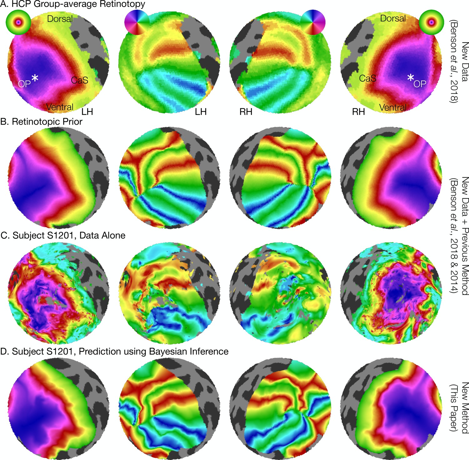
The retinotopic prior and its use in predicting retinotopic maps.
(A) The retinotopic prior is based on the Human Connectome Project (HCP) group-average retinotopic maps (Benson et al., 2018), shown here on an orthographic projection of the V1-V3 region. OP indicates the occipital pole, and CaS indicates the Calcarine sulcus. Projections are identical in each row throughout. (B) The retinotopic prior was designed to resemble the HCP group-average retinotopy, and was further warped to minimize differences between the two according to the methods described by Benson et al. (2014). (C) The measured (‘Data Alone’) retinotopic maps of subject S1201, all scans combined. Comparison of rows B and C demonstrates that the use of the retinotopic prior to predict the retinotopic maps of an individual subject results in a reasonable prediction. (D) Combining the retinotopic prior with the observed retinotopic maps from an individual subject yields Bayesian inferred maps.
Figure 3
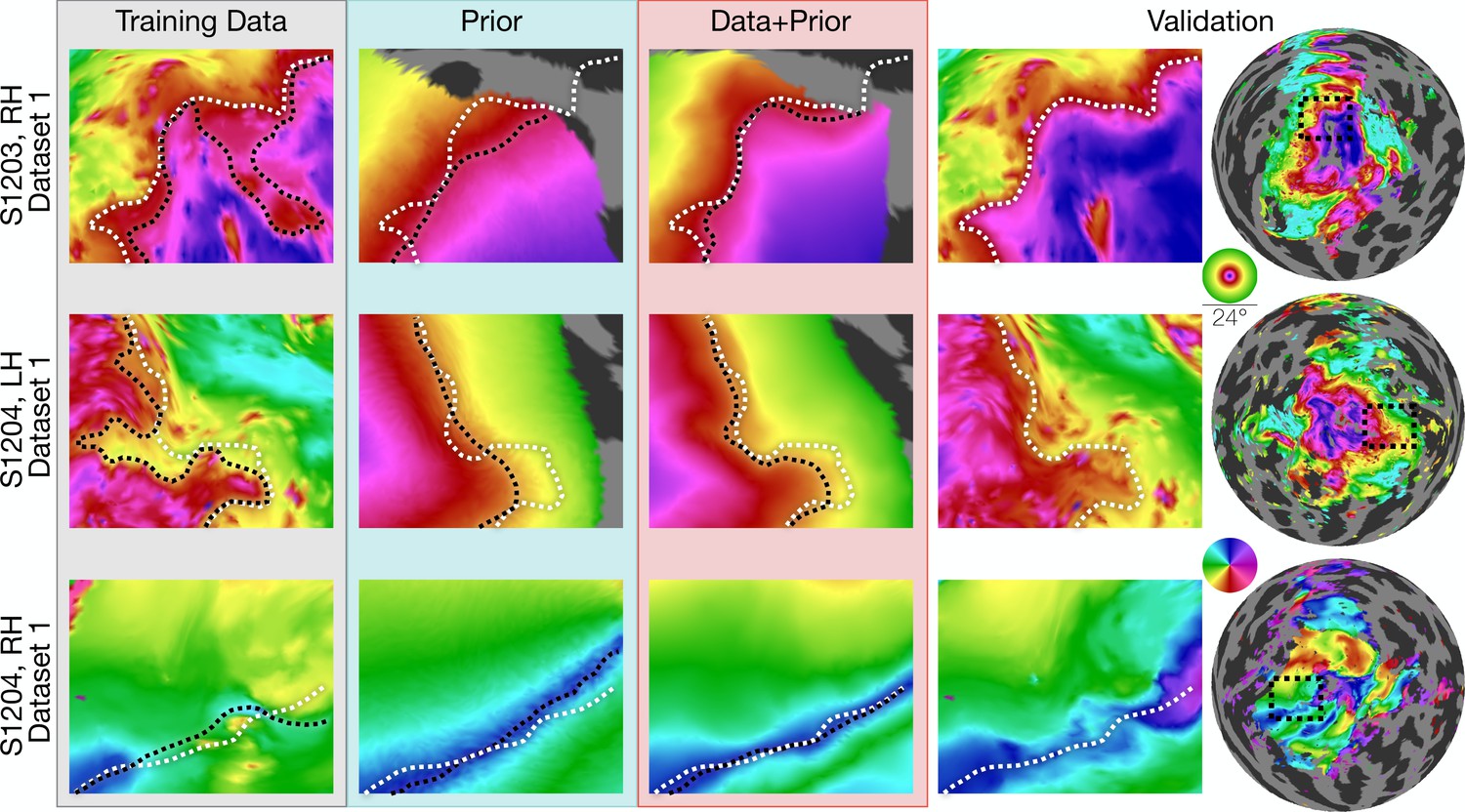
Inferred retinotopic maps accurately predict features of validation retinotopy.
Twelve close-up plots of the retinotopic maps of three hemispheres are shown with predictions made from Data alone, Prior alone, or Data +Prior. The right two columns show the validation dataset with the right column indicating the context of the close-up patches. The first three columns show different methods of predicting the retinotopic maps, as in Figure 1. Approximate iso-eccentricity or iso-angular contour lines for the validation dataset have been draw in white on all close-up plots. Black contour lines show the same approximate contour lines for the three prediction methods. Flattened projections of cortex were created using an orthographic projection (Supplementary file 2A).
Figure 4
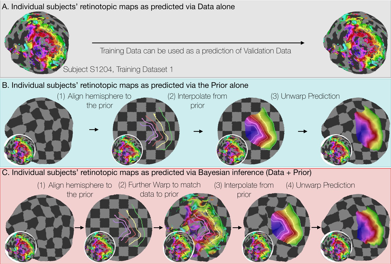
Deriving retinotopic predictions.
Three methods of predicting retinotopic maps (as in Figure 1) for an example subject. (A) Predicted retinotopic maps based on training data alone are found by solving the pRF models for each voxel and projecting them to the cortical surface. The training data (left) and prediction (right) are identical. (B) To predict a retinotopic map using the prior alone, the subject’s cortical surface is aligned to FreeSurfer’s fsaverage anatomical atlas (represented by rectilinear checkerboards), bringing the subject’s anatomy into alignment with the anatomically-based prior, which is represented by iso-eccentricity contour lines in the figure (see also Supplementary file 2C). The model of retinotopy is then used to predict the retinotopic parameters of the vertices based on their anatomically-aligned positions. After the predictions have been made, the cortical surface is relaxed. Maps are shown as checkerboards in order to demonstrate the warping (insets show original data and curvature). (C) Bayesian inference of the retinotopic maps of the subject are made by combining retinotopic data with the retinotopic prior. This is achieved by first aligning the subject’s vertices with the fsaverage anatomical atlas (as in B) then further warping the vertices to bring them into alignment with the data-driven model of retinotopy (shown as iso-eccentricity contour lines). The warping was performed by minimizing a potential function that penalized both the deviation from from the prior (second column) as well as deviations between the retinotopic observations and the retinotopic model.
Figure 5
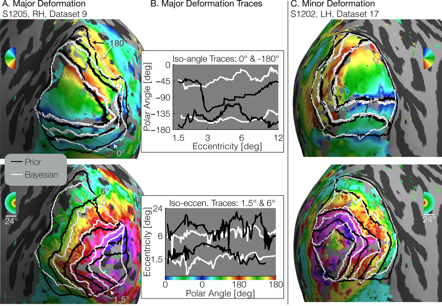
Comparison of inferred and prior maps.
(A) A subject whose maps were poorly predicted by the retinotopic prior and thus required major deformation (S1205, RH, dataset 9). (B) To illustrate the differences between the Prior Alone (black lines in A) and the combination of Data +Prior (white lines in A), traces of the polar angle (top) and eccentricity (bottom) values beneath the lines indicated by arrows are shown. The eccentricities traced by the iso-angle lines and the polar angles traced by the iso-eccentricity lines of the Bayesian-inferred maps more closely match the angles/eccentricities of their associated trace lines than do the polar angles/eccentricities beneath the lines of the Prior alone (C) A subject whose retinotopic maps were well-predicted by the prior and thus required relatively minor deformation during the Bayesian inference step (subject S1202, LH, dataset 17). In both A and C, black lines show the retinotopic prior and white lines show the maps inferred by Bayesian inference.
Figure 6
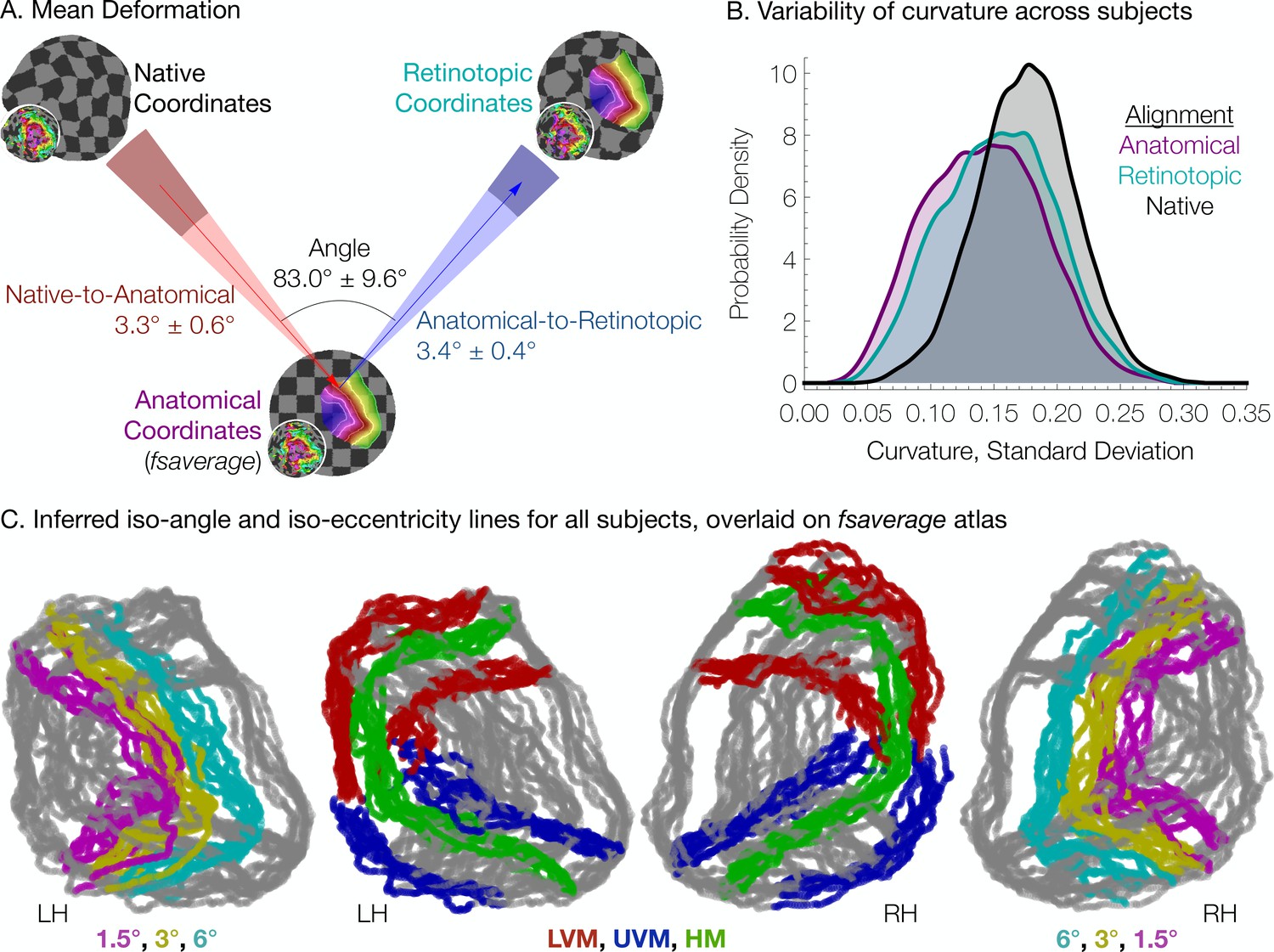
Individual differences between subjects in the structure-function relationship are substantial.
(A) The mean deformation vectors, used to warp a surface vertex from its Native to its Anatomical (fsaverage-aligned) position and from its Anatomical to its Retinotopic position, are shown relative to each other. The wedges plotted beneath the mean arrows indicate ±1 standard deviation of the angle across subjects while the shaded regions at the end of the wedges indicate ±1 standard deviation of the lengths of the vectors. Note that because registration steps are always performed on a subject's inflated spherical hemispheres, these distances were calculated in terms of degrees of the cortical sphere and are not directly equivalent to mm of cortex. (B) The alignment of the V1-V3 region to the retinotopic prior increases the standard deviation of the surface curvature across subjects, suggesting that retinotopic alignment is not simply an improvement on FreeSurfer’s curvature-based alignment. Histograms show the probability density of the across-subject standard deviation of curvature values for all vertices in the V1-V3 region with a Bayesian-inferred eccentricity between 0 and 12°. (C) Bayesian-inferred iso-eccentricity lines and V1/V2/V3 boundaries plotted for all subjects simultaneously on the fsaverage spherical atlas. Lines are plotted with an opacity of 1/2 to visualize overlap. The left two plots and the right two plots share identical lines but have different colors. Iso-eccentricity lines are colored in magenta (1.5°), yellow (3°), and cyan (6°). Iso-angle lines are plotted in blue (upper vertical meridian), green (horizontal meridian), and red (lower vertical meridian).
Figure 7
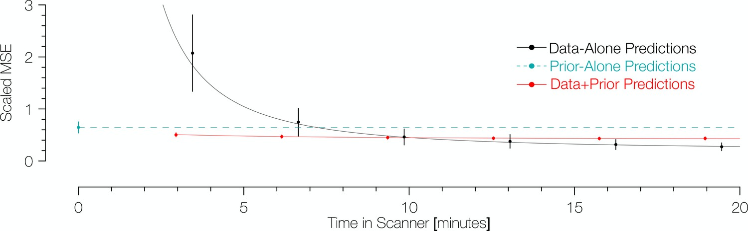
Comparison of prediction errors for three methods of predicting retinotopic maps.
Errors are shown in terms of the number of minutes spent collecting retinotopic mapping scans (x-axis). The y-axis gives the mean squared eccentricity-scaled error. Each plotted point represents a different number of minutes in the scanner, with error bars plotting ±1 standard error across subjects. For short scan times, errors are significantly higher for predictions made with the data alone than for those made using Bayesian inference. An offset has been added to the x-values of each of the black (−0.25) and red (+0.25) points to facilitate viewing.
Figure 8
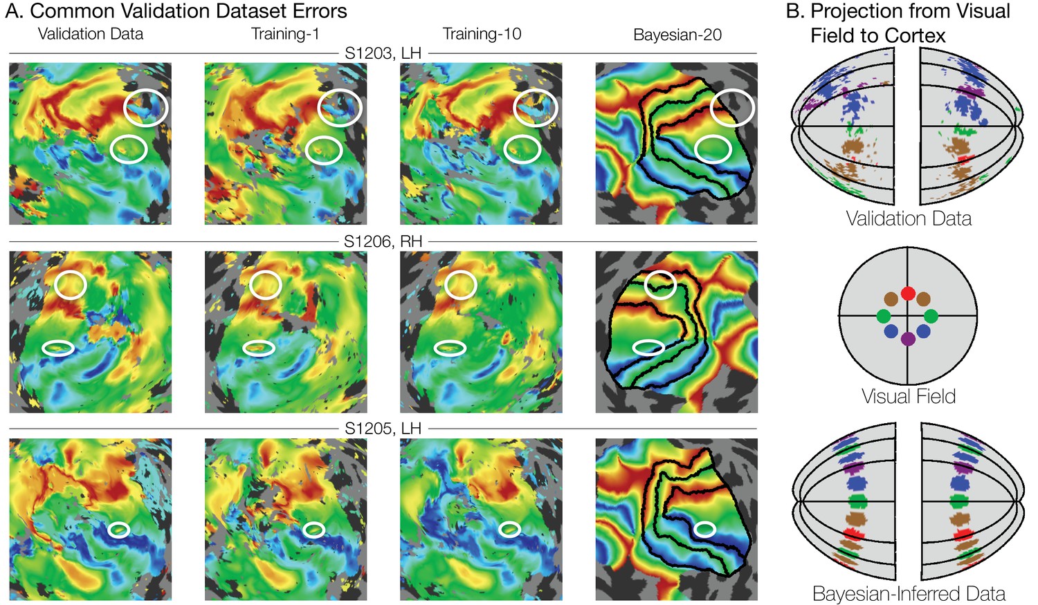
Systematic errors in training and validation datasets.
(A) Many small inconsistencies in the retinotopic maps are duplicated in both the validation dataset and the training datasets but not in the maps predicted by Bayesian inference. Maps for three example hemispheres are shown with validation datasets as well as training dataset 1, training dataset 10, and the Bayesian-inferred maps from dataset 20. Ellipses highlight blips of noise in the validation maps that are unlikely to represent the true underlying map, but that are correlated with the training maps. Such blips are significantly different in the inferred and validation maps, likely inflating the error of the inferred maps. Black lines show the V1-V3 boundaries in the Bayesian-inferred maps. (B) Discontinuity errors. If the validation data is used to project the disks shown in the visual field in the middle panel to the cortical surface, the resulting map is messy and contains a number of inconsistencies due to measurement error. While the Bayesian inferred map may contain errors of its own, it will always predict a topologically smooth retinotopic map with respect to the topology of the visual field.
Figure 9
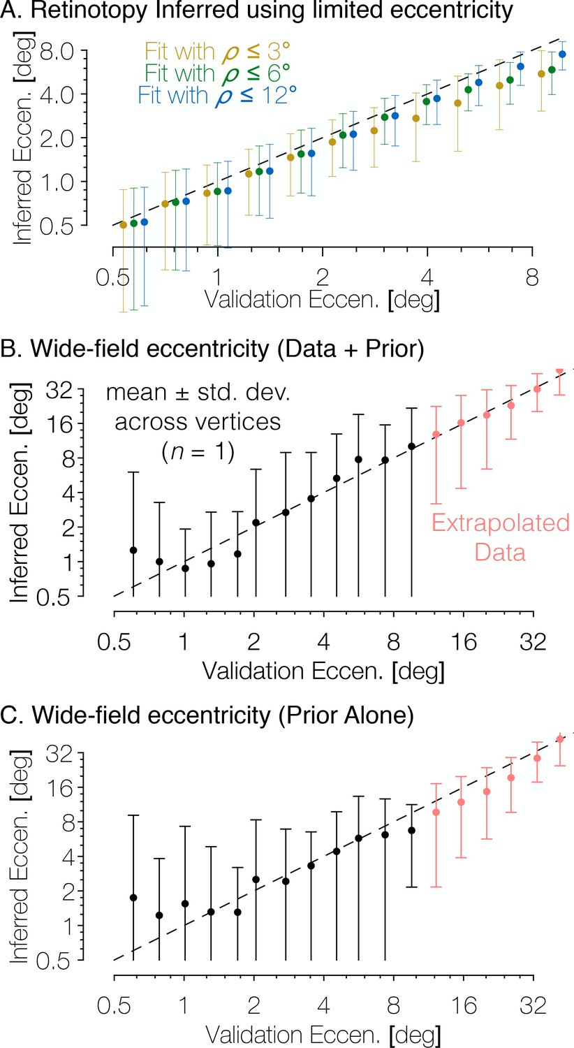
The Bayesian-inferred maps accurately predict eccentricity beyond the range of the stimulus.
(A) In order to examine how accurately the retinotopic maps predicted using Bayesian inference describe the retinotopic arrangement outside of the range of the stimulus used to construct them we constructed maps from all datasets using only the inner 3° or 6° of eccentricity then compared the predictions to the full validation dataset. Eccentricity is well predicted out to 12° regardless of the eccentricity range used to construct the predicted map, indicating that our inferred maps are likely accurate beyond the range of the stimulus. In addition, we compared the wide-field retinotopic mapping data from subject S1201 to the inferred retinotopic maps (B) and the anatomical prior (C) using only the 12° stimulus; the inferred eccentricity is shown in terms of the validation eccentricity. The highest errors appear in the fovea (<3°), while predictions made by the inferred maps are most accurate in the periphery, indicating that eccentricity may be well-predicted far beyond the range of the stimulus (out to 48° of eccentricity in this case). Predictions of peripheral data are slightly less accurate when made by the prior than by the inferred maps, which suggests that the extrapolation is improved by the Bayesian inference.
Figure 10

Aggregate pRF size and cortical magnification measurements are in agreement with previous literature.
(A) PRF sizes by eccentricity are shown for V1, V2, and V3, as calculated from the full datasets; shaded regions show standard errors across subjects. (B) Cortical magnification is shown in terms of eccentricity for V1-V3, as calculated from the full datasets. Again, the shaded regions show standard errors across subjects. The dashed black line shows the equation for cortical magnification provided by Horton and Hoyt, 1991. (C) Cortical magnification as calculated using the pRF coordinates inferred by the Bayesian inference. Note that in both A and B, eccentricity refers to measured eccentricity while in C, eccentricity refers to Bayesian-inferred eccentricity. (D) The difference between the cortical magnification predicted by Horton and Hoyt, 1991 and the cortical magnification of the (D) measured and (E) inferred maps; the data are the same as in B and C.
Tables
Table 1
Summary statistics for each subject.
https://doi.org/10.7554/eLife.40224.008| Subject | Hemisphere | V1 area (mm3)* | V1 volume (mm3)* | Anatomical RMSD† | Retinotopic RMSD† |
|---|---|---|---|---|---|
| S1201 | RH | 1308 | 3733 | 2.88 | 3.15 |
| S1201 | LH | 1315 | 4133 | 1.82 | 2.47 |
| S1202 | RH | 2024 | 3706 | 1.21 | 2.73 |
| S1202 | LH | 2085 | 4199 | 1.28 | 2.65 |
| S1203 | RH | 1574 | 3152 | 2.13 | 3.27 |
| S1203 | LH | 1489 | 2941 | 2.06 | 3.77 |
| S1204 | RH | 1906 | 3325 | 2.29 | 3.00 |
| S1204 | LH | 1645 | 3015 | 2.18 | 3.10 |
| S1205 | RH | 1995 | 3926 | 1.99 | 2.91 |
| S1205 | LH | 1884 | 3372 | 1.76 | 3.31 |
| S1206 | RH | 1647 | 3116 | 2.12 | 2.73 |
| S1206 | LH | 1632 | 2692 | 1.63 | 3.22 |
| S1207 | RH | 1648 | 3402 | 1.84 | 2.41 |
| S1207 | LH | 1421 | 2764 | 1.74 | 3.15 |
| S1208 | RH | 1712 | 3509 | 1.50 | 2.58 |
| S1208 | LH | 1494 | 3083 | 1.89 | 3.08 |
-
* The V1 boundary was determined from the Bayesian-inferred map constructed by combining the retinotopic prior with the full retinotopy dataset.
† Units of the RMSD values are degrees of the cortical sphere; these are approximately equivalent to mm, but exact measurements in mm are distorted during inflation of the surface. ‘Anatomical’ RMSD refers to the deviation between the subject’s native anatomical sphere and the fsaverage-aligned sphere while ‘Retinotopic’ RMSD refers to the deviation between the fsaverage-aligned sphere and the retinotopically aligned sphere. The RMSD values were averaged over all vertices within the inner 12° of eccentricity of the V1-V3 region. Use of a larger patch of cortex (e.g., the flattened map projections in Figure 4A) does not qualitatively change the relationship between anatomical and retinotopic RMSD values.
Table 2
Components of the registration potential function
https://doi.org/10.7554/eLife.40224.013| Term | Description | Form | |
|---|---|---|---|
| 1 | Penalizes changes in the distances between neighboring vertices in the mesh. | ||
| 2 | Penalizes the changes in t he angles of the triangles in the mesh. | ||
| 3 | Penalizes any change in the positions of the vertices on the perimeter of the map. | ||
| 4 | Decreases as a retinotopic vertex u approaches its anchor-point y in the retinotopy model. | ||
| 5 | Harmonic component of the edge-length deviation penalty . | ||
| 6 | Infinite-well component of the edge-length deviation penalty . | ||
| 7 | Harmonic component of the angle deviation penalty . | ||
| 8 | Infinite-well component of the angle deviation penalty . |
Additional files
-
Supplementary file 1
Cross-validation schema.
To evaluate the accuracy of the predictions of retinotopic maps, we employ a cross-validation schema. Each subject’s 12 retinotopic mapping scans were divided into one large set of validation data as well as 21 smaller sets of training data. An additional dataset of all 12 scans was used for analysis of retinotopic properties not linked to evaluation of the quality of the predicted maps.
- https://doi.org/10.7554/eLife.40224.014
-
Supplementary file 2
Deriving the anatomically-defined atlas of retinotopy (the prior).
(A) The group-average polar angle (top) and eccentricity (bottom) maps. The cortical surface is inflated to a sphere then flattened to a map. (B) The model of retinotopy shown with polar angle plotted on the left and eccentricity plotted on the right hemispheres. (C) The retinotopic prior is constructed from the group-average data using an updated version of the method described by Benson et al. (2014). Note that while only eccentricity is shown, polar angle and eccentricity are registered simultaneously. The checkerboard underlay illustrates the anatomical warping. (D) There is approximate agreement between the boundaries of visual areas V1, V2, and V3 as defined by two atlases. The Wang et al. maximum probability atlas (2015) and the retinotopic template defined here have similar boundaries. The template extends from 0° to 90° eccentricity, whereas the Wang et al atlas is limited to the field of view of their experiments (14°), hence the template maps are larger. (E) Because there is a topological isomorphism between the cortical surface, the left and right hemifields, and the model of retinotopy, the three representations have exact one-to-one correspondences.
- https://doi.org/10.7554/eLife.40224.015
-
Supplementary file 3
The retinotopic prior.
(A) The 181-subject group-average retinotopic maps from the Human Connectome Project 7T Retinotopy Dataset are shown. These maps were used to construct the prior. Black arrows in the left-most plots indicate ‘notches’ of the V3 representation of the upper and lower vertical meridians that are absent in the group-average data. (B) The retinotopic prior is shown from 0 to 12° of eccentricity with boundary lines between areas. All 12 retinotopic areas included in the prior are shown.
- https://doi.org/10.7554/eLife.40224.016
-
Supplementary file 4
Warp fields in the V1-V3 region across all subjects.
The warp fields are calculated using the individual vertex deviations during the registration process (Figure 3C). The top row shows the mean vertex deformation across all subjects while the bottom three rows show the first three principal components of the deviations. The brightness of the arrows is based on their relative lengths. Note that because the top row shows the mean warp-field across subjects, the exact direction of the arrows is significant; however, in the bottom three rows, the principal component axes are shown, so the inversion of the arrows is equivalent to the plotted arrows.
- https://doi.org/10.7554/eLife.40224.017
-
Supplementary file 5
Retinotopic maps for subjects
(A) 198653 and (B) 644246 from the Human Connectome Project. These two subjects have unusual retinotopic organization in the polar angle maps of their left hemispheres (A) and on both hemispheres (B); this organization is not accounted for my our model of retinotopy and thus provides an example of how our Bayesian inference method performs when provided with atypical retinotopic maps. In the polar angle maps (top), black lines indicate V1/V2/V3 boundaries. In the eccentricity maps (bottom), black lines show the outer V3 boundaries and the 0.5°, 1°, 2°, 4° and 8° iso-eccentricity curves. Black arrows indicate the sites of atypical retinotopic organization.
- https://doi.org/10.7554/eLife.40224.018
-
Transparent reporting form
- https://doi.org/10.7554/eLife.40224.019
Download links
A two-part list of links to download the article, or parts of the article, in various formats.
Downloads (link to download the article as PDF)
Open citations (links to open the citations from this article in various online reference manager services)
Cite this article (links to download the citations from this article in formats compatible with various reference manager tools)
Bayesian analysis of retinotopic maps
eLife 7:e40224.
https://doi.org/10.7554/eLife.40224


