Bumblebee visual allometry results in locally improved resolution and globally improved sensitivity
- Lund University, Sweden
- Westphalian University of Applied Sciences, Germany
- Diamond Light Source, United Kingdom
- Stockholm University, Sweden
Figures
Figure 1
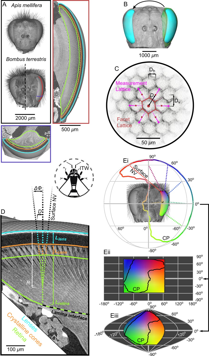
Tomographic images of bee eyes and visual analysis.
(A) Volume rendering of the dried heads of workers from the bee species used in this study. The right-hand side of a small B. terrestris head is shown (intertegular width (ITW) = 3.0 mm) in comparison to left hand side of a large individual from the same colony (ITW = 5.4 mm, note that the mandibles and some hair of this bee were too large to image). The ITW of the A. mellifera specimen was 3.6 mm. The box on the right displays a vertical section along the midline of a B. terrestris apposition compound eye showing the gross morphology of the lenses, crystalline cones (CC), and retina (indicated using colored outlines as in panel D). A portion of the optic lobe is also visible to the left of the retina. The lower box shows a transverse section across the ventral portion of the compound eye, showing the same features as in the vertical section. The approximate location of the sections are indicated with lines on the larger B. terrestris eye; both sections have the same scaling. (B) A volume rendering of the left compound eye (green) of each bee was aligned onto a rendering of the full head of another bee (grey), which allowed the segmented eye (cyan) to be placed relative to the head and also mirrored to the right side. (C) To measure the local facet dimensions, six points were selected on the opposing borders of the six facets that surrounded a central facet. These points were then used to compute the local structure of the facet lattice from which the lens diameter D was calculated (the horizontal (Dh) and vertical (Dv) facet dimensions were not used in this study). (D) Surface normal vectors (NV) were calculated from the exterior surface of the lenses to indicate the local viewing direction. The IF angle (ΔΦ) was defined as the difference between viewing directions at a distance of one lens diameter. The NV was traced into the eye and the points where it intersected the front surface of the CC, the retina, and the lamina interface were used to determine the thickness of these structures (Llens, Lcone, and Lretina, respectively). Note that the angle of the CC and the photoreceptors in the retina can be misaligned from the corneal NV, in which case the IF can differ from the IO angle. Inset, a diagram shows the measurement of ITW as the distance between the wing bases on a bee’s thorax. (Ei) The projection of the NVs (several are plotted as dotted lines) from the eye onto a sphere indicates the extent of the eye’s corneal projection (CP), which can also be represented on equirectangular (ii) or sinusoidal (iii) projections on which the CP is indicated by black lines. The color coding indicates the viewing direction, and was applied by stretching a 2D color map across the CP extent on the equirectangular projection in (ii); equivalent colors indicate the same viewing direction in each projection.
Figure 2
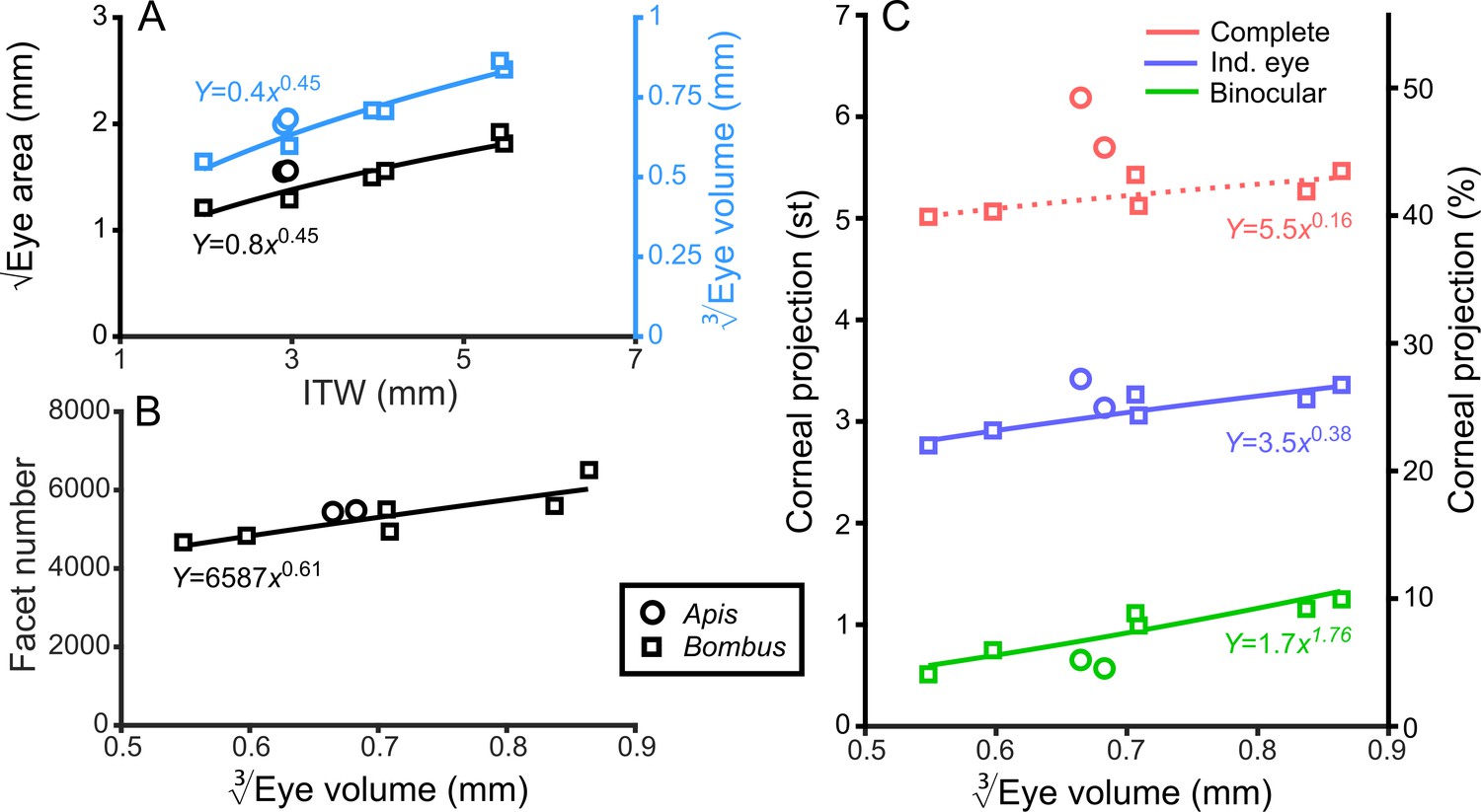
General analysis of differently sized compound eyes.
(A) √Eye area and (on the right-hand Y-axis) vs. ITW. (B) The number of facets in each compound eye as a function of . (C) The size of the individual (Ind.), binocular, and complete CPs both in steradians (left Y-axis, max.: 4π) and as a percentage of the total visual sphere (right Y-axis, max.: 100%). Squares denote bumblebees whereas circles denote honeybees in all plots, while color coding is explained on each panel. A power function was fitted to the Bombus measurements for each parameter (Supplementary file 1–Table S1); the resulting functions are written and plotted in each panel. The dotted line in panel C indicates that the correlation between the complete CP and was not significant.
Figure 3 with 5 supplements
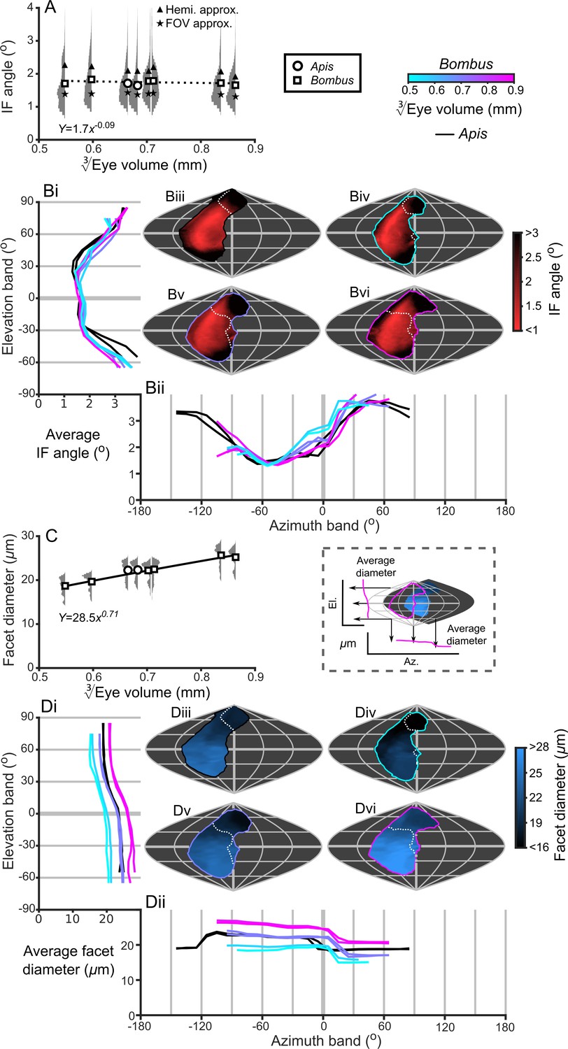
IF angle and facet diameter averages and projections.
(A) Average IF angles and relative distribution of IF angles for each bee. The triangles indicate the results of dividing a hemisphere by the total facet number to predict the average IF angle (Hemi. approx.) (Land, 1997), while the stars indicate the results of dividing an individual eye’s angular CP by its total facet number (FOV approx.). (B) The topographic distribution of IF angle (indicated by the red-black color gradient bar) projected from each bee’s eye, shown as sinusoidal projections for a honeybee (iii) and for small- (iv), medium- (v) and large-sized (vi) bumblebees (azimuth and elevation lines are plotted at 60° and 30° intervals, respectively). Profiles of the average IF angle are shown for elevation (panel Bi, where IF angle is averaged across all azimuth points in each eye’s CP) and azimuth (panel Bii, where IF angle is averaged across all elevation points in each eye’s CP). The diagram below panel Bii provides a graphical representation of averaging topologies to profiles. (C) Averages and relative distributions of the facet diameters from each bee (bees as in panel A). (D) As for panel B but showing the topology (indicated by the blue-black color gradient bar) and profiles of average facet diameter. Squares denote bumblebees and circles denote honeybees in panels A and C, and a power function was fitted to the Bombus measurements for the parameters in these panels (Supplementary file 1–Table S1); the resulting functions are written and plotted in each panel. The dotted line in panel A indicates that the correlation between the IF angle and was not significant. The cyan-to-magenta color bar indicates the of the Bombus profiles in panels B and D, while black lines indicate honeybees. The white dotted lines across the topologies in panels B and D (iii to vi) indicate the border of a bee’s binocular CP. See Figure 3—figure supplements 1–4 for equivalent data on curvature, lens and crystalline cone thickness, and eye parameter. Correlations between each locally measured variable are plotted in Figure 3—figure supplement 5.
Figure 3—figure supplement 1
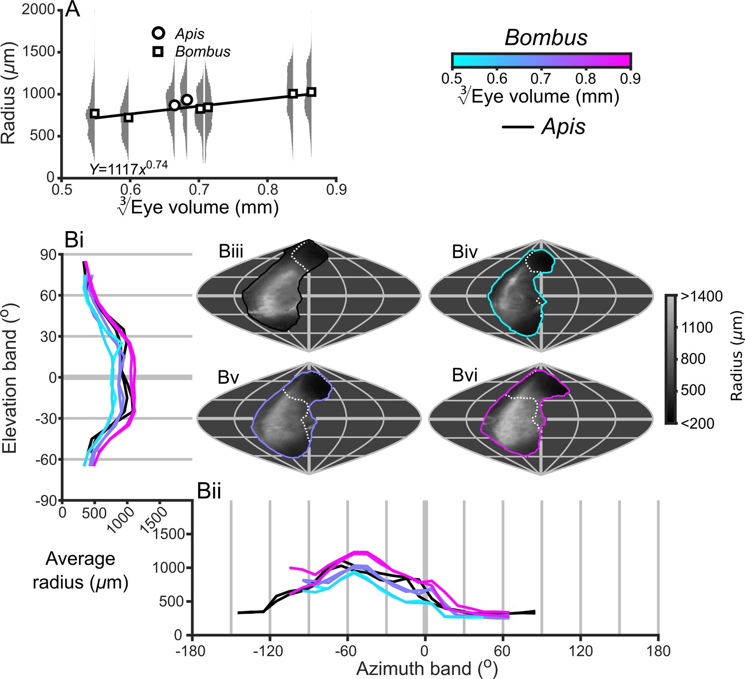
Description of the local radius of the curvature of compound eyes.
(A) The average radii and relative distribution for each bee vs. EV. The plotted curve results from fitting the function parameters to the measurements for Bombus (additional details in Supplementary file 1–Table S1). (B) The topographic distribution of R (indicated by the grey color gradient bar) projected from each bee into the visual world, shown as sinusoidal projections for a honeybee (iii), and for small- (iv), medium- (v) and large-sized (vi) bumblebees (azimuth and elevation lines are plotted at 60° and 30° intervals, respectively). Profiles of average radii are shown for elevation (panel Bi, R is averaged across all azimuth points in each eye’s CP as function of elevation) and azimuth (panel Bii, R is averaged across all elevation points in each eye’s CP as a function of azimuth). The white dotted lines across the topology in panels Biii to Bvi indicate the border of the bee’s binocular CP. The cyan-to-magenta color bar indicates the of Bombus for each curve in all panels, whereas black lines indicate honeybees.
Figure 3—figure supplement 2
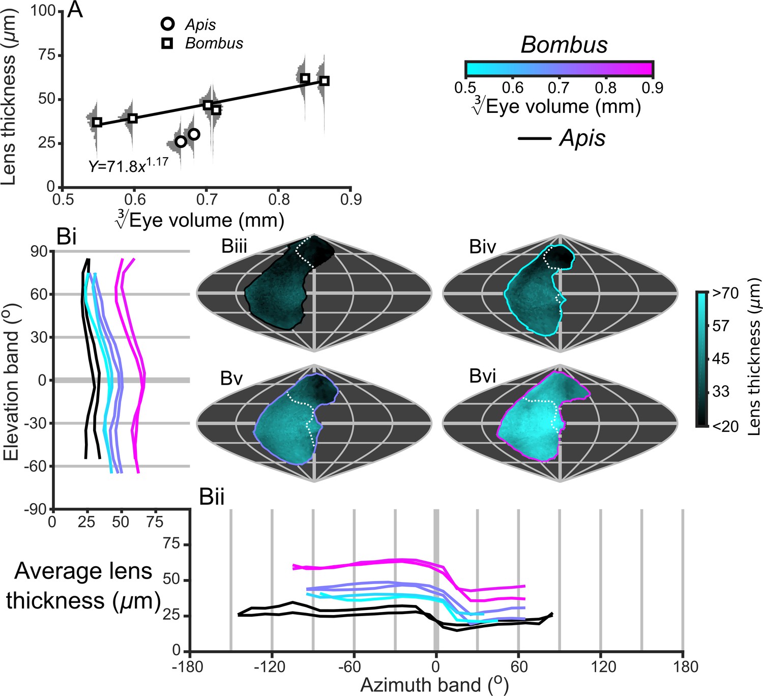
Description of the local lens thickness of compound eyes.
(A) The average lens thickness and relative distribution for each bee vs. EV. The plotted curve results from fitting the function parameters to the measurements for Bombus (additional details in Supplementary file 1–Table S1). (B) The topographic distribution of lens thickness (indicated by the cyan color gradient bar) projected from each bee into the visual world, shown as sinusoidal projections for a honeybee (iii), and for small- (iv), medium- (v), and large-sized (vi) bumblebees (azimuth and elevation lines are plotted at 60° and 30° intervals, respectively). Profiles of the average lens thickness are shown for elevation (panel Bi, thickness is averaged across all azimuth points in each eye’s CP as a function of elevation) and azimuth (panel Bii, thickness is averaged across all elevation points in each eye’s CP as a function of azimuth). The white dotted lines across the topology in Biii to Bvi indicate the border of the bee’s binocular CP. The cyan-to-magenta color bar indicates of Bombus for each curve in all panels, whereas black lines indicate honeybees.
Figure 3—figure supplement 3
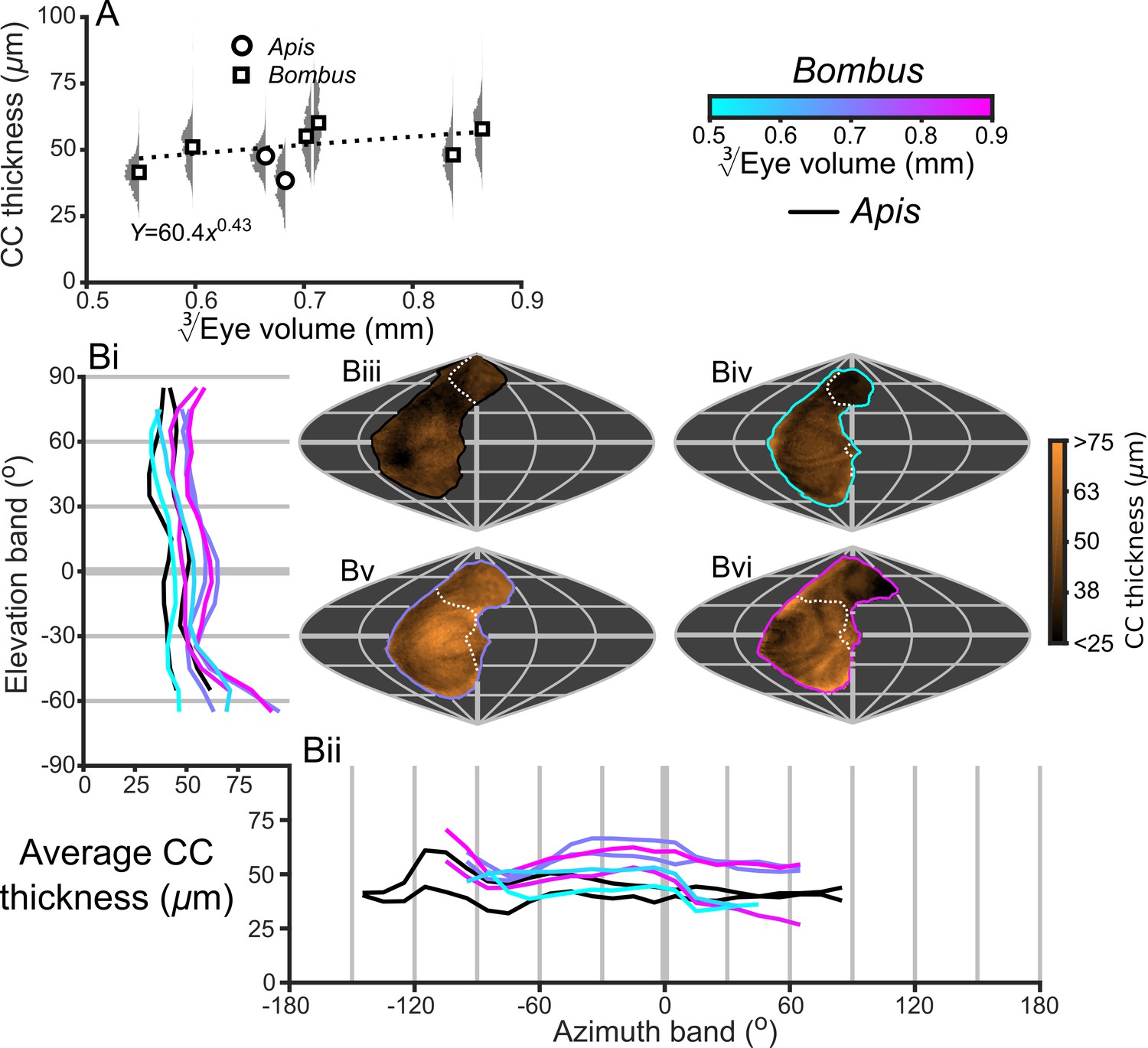
Description of the local CC thickness of compound eyes.
(A) The average CC thickness and relative distribution for each bee vs. . The plotted curve results from fitting the function parameters to the measurements for Bombus (additional details in Supplementary file 1–Table S1), however, the correlation between CC thickness and is not significant. (B) The topographic distribution of CC thickness (indicated by the orange color bar) projected from each bee into the visual world, shown as sinusoidal projections for a honeybee (iii), and for small- (iv), medium- (v), and large-sized (vi) bumblebees (azimuth and elevation lines are plotted at 60° and 30° intervals, respectively). Profiles of the average CC thickness are shown for elevation (panel Bi, thickness is averaged across all azimuth points in each eye’s CP as a function of elevation) and azimuth (panel Bii, thickness is averaged across all elevation points in each eye’s CP as a function of azimuth). The white dotted lines across the topology in Biii to Bvi indicate the border of the bee’s binocular CP. The cyan-to-magenta color bar indicates the of Bombus for each curve in all panels, whereas black lines indicate honeybees.
Figure 3—figure supplement 4
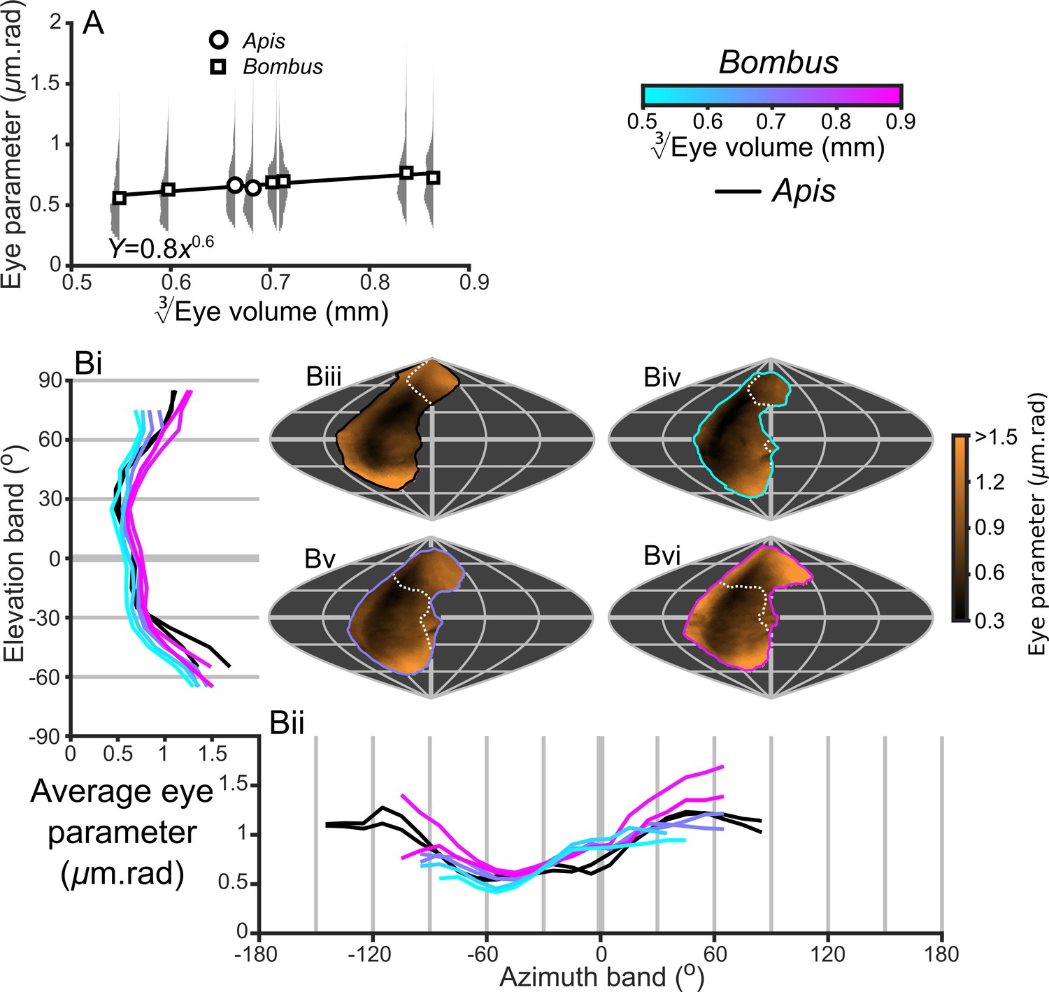
Description of the local eye parameter of compound eyes.
(A) The average eye parameters and relative distribution for each bee vs. EV. The plotted curve results from fitting the function parameters to the measurements for Bombus (additional details in Supplementary file 1–Table S1). (B) The topographic distribution of eye parameter (indicated by the orange color bar) projected from each bee into the visual world, shown as sinusoidal projections for a honeybee (iii), and for small- (iv), medium- (v) and large- sized (vi) bumblebees (azimuth and elevation lines are plotted at 60° and 30° intervals, respectively). Profiles of average eye parameter are shown for elevation (panel Bi, eye parameter is averaged across all azimuth points in each eye’s CP as function of elevation) and azimuth (panel Bii, eye parameter is averaged across all elevation points in each eye’s CP as a function of azimuth). The white dotted lines across the topology in Biii to Bvi indicate the border of the bee’s corneal binocular CP. The cyan-to-magenta color bar indicates the of Bombus for each curve in all panels, whereas black lines indicate honeybees. Note that we used the calculated IF angle (Figure 3B) in place of the IO angle when calculating the eye parameter.
Figure 3—figure supplement 5
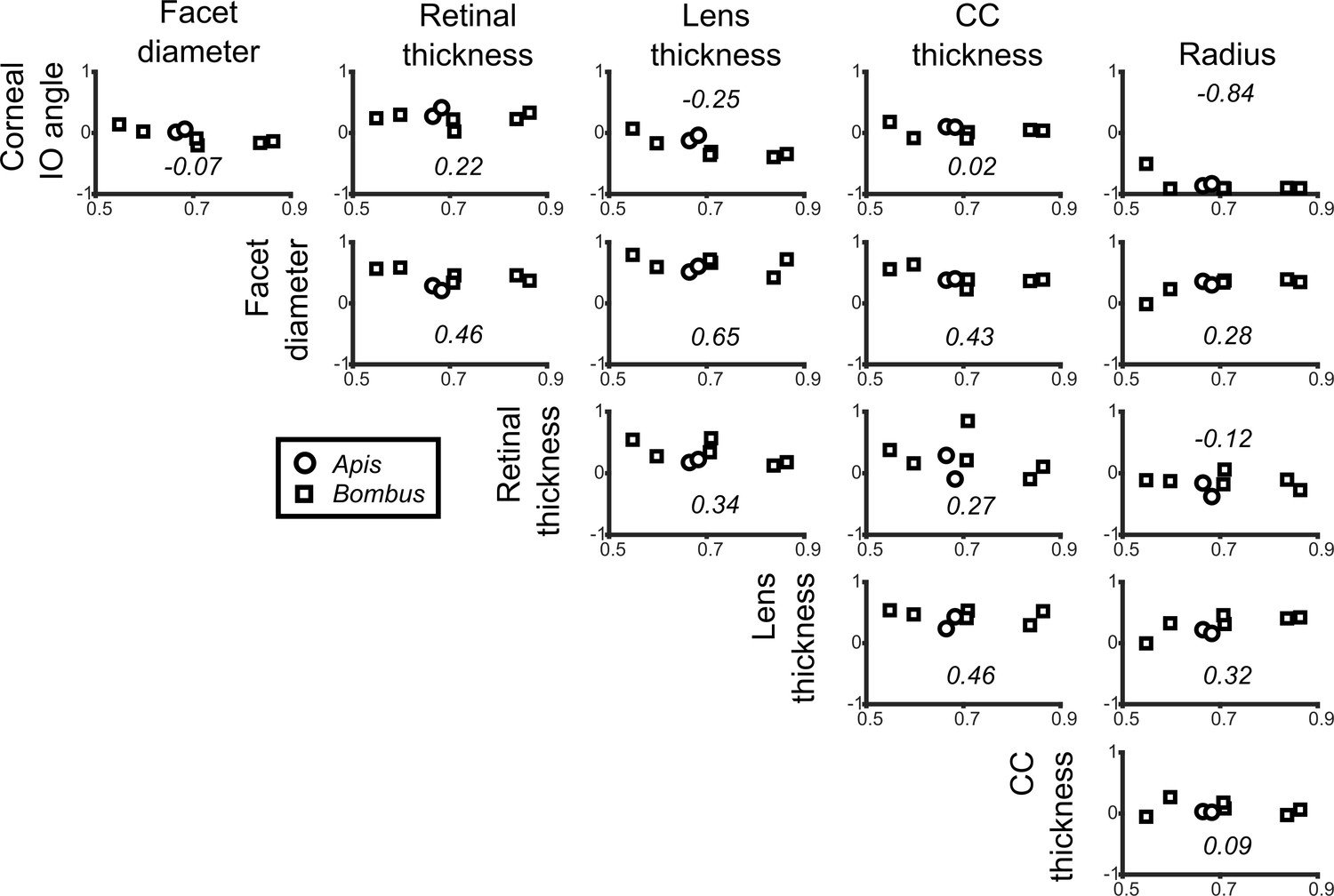
Correlation of local variable values.
The matrix of graphs representing the correlation coefficient (r) between two local variables, measured for each bee vs. . The vertically oriented variable names for each row are cross-referenced against the horizontally oriented variable names for each column to determine the correlation shown in each plot. The italicized number in each plot represents the average of that plot’s correlation coefficient for all bees.
Figure 4
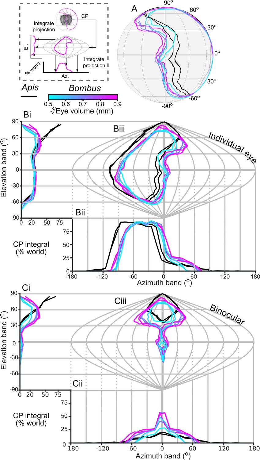
The corneal projection (CP) of compound eyes.
(A) The CP of each bee’s left eye shown on a sphere representing the world. (B) A sinusoidal projection and analysis of the CPs (iii). Profiles of integrated CP are shown across elevation (panel Bi, the integral of all azimuth points in the CP as a function of elevation) and azimuth (panel Bii, the integral of all elevation points in the CP as a function of azimuth) and are expressed as a percentage of the total number of points. (C) As for panel B but depicting the limit of the binocular overlap between the visual field of the left and right eyes for each bee. Colouring of the CP and profile lines is indicated by the color gradient bar as described in the caption of Figure 3. See Figure 1E for a visualization of the relationship between a sphere and its projections and the diagram to the left of panel A for a graphical representation of integrating CPs to profiles.
Figure 5 with 1 supplement
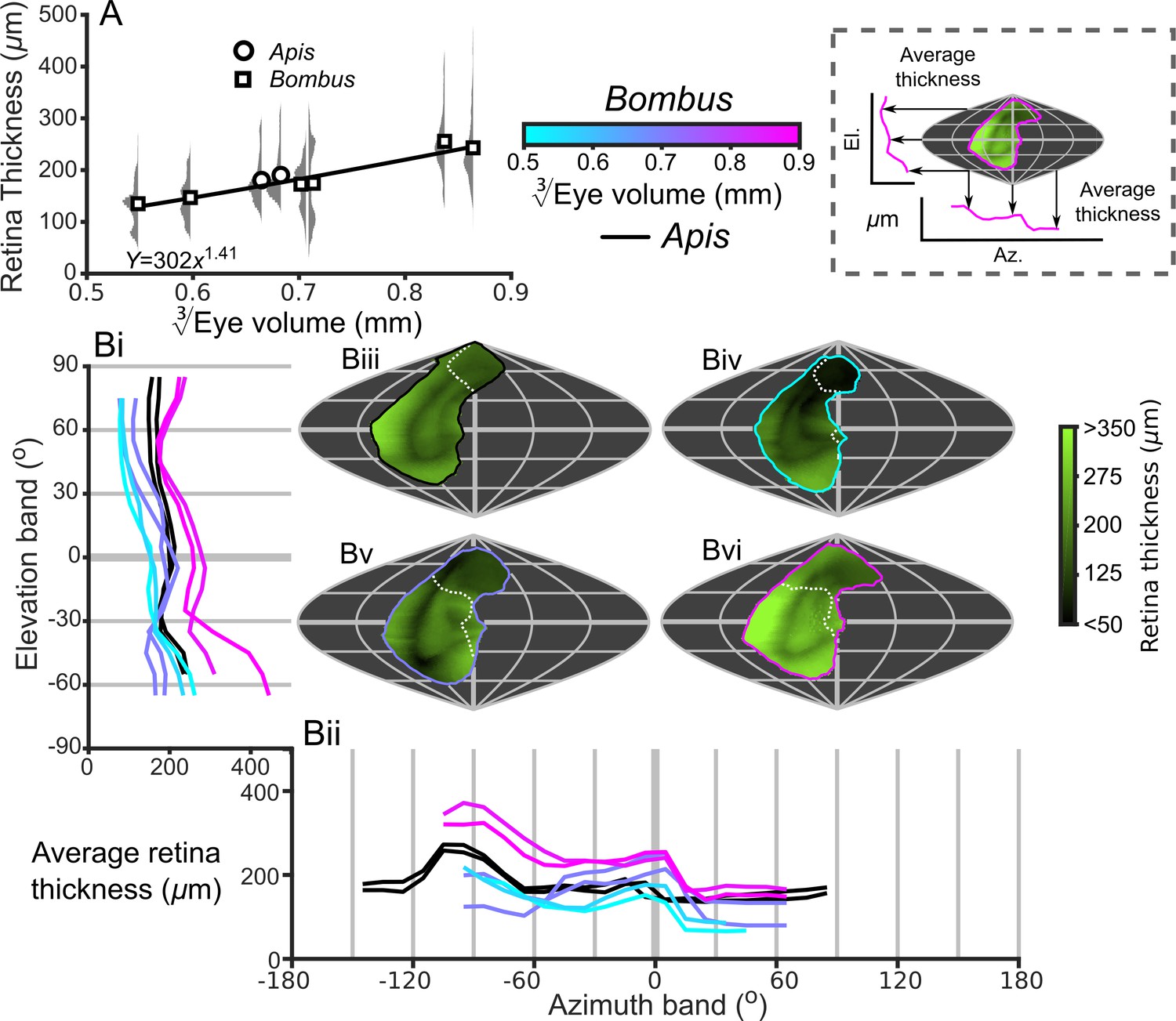
Description of the retinal thickness underlying compound eyes.
(A) The average retinal thicknesses and relative distribution for each bee as a function of (notes in the caption for Figure 2 also apply to this panel). (B) The topographic distribution of retinal thickness (indicated by the green-black color gradient bar) projected from each bee into the visual world, shown as sinusoidal projections for a honeybee (iii), and for small- (iv), medium- (v), and large-sized (vi) bumblebees. Profiles of the average retinal thickness are shown for elevation (panel Bi, where thickness is averaged as a function of elevation, as described in the caption for Figure 3B) and azimuth (panel Bii, thickness is averaged as a function of azimuth). Further details about projections and profiles are described in the caption of Figure 3. The average calculated sensitivity for each eye is show in Figure 5—figure supplement 1.
Figure 5—figure supplement 1
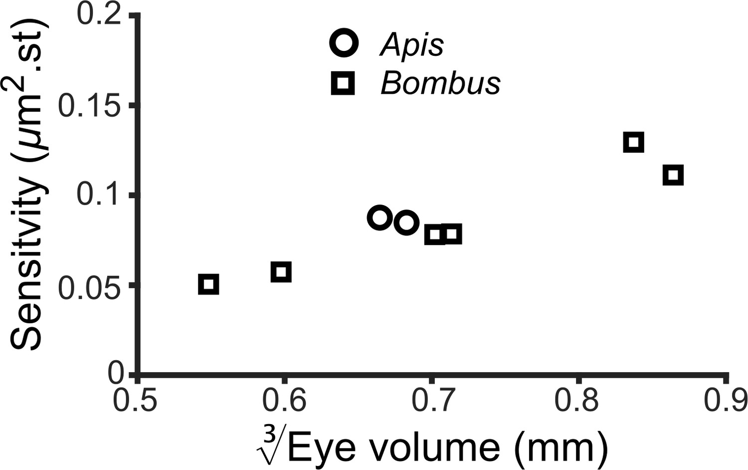
The average optical sensitivity calculated for each bee vs .
Note that this calculation assumes that the acceptance angle of each facet equals its IF angle and that the rhabdom length equals the retinal thickness and should be treated as an approximation.
Figure 6 with 1 supplement
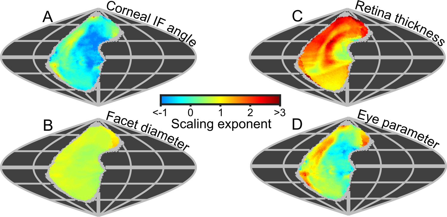
Eye metrics and maps of scaling exponents in the visual world.
(A–D) Maps of the scaling exponents calculated for bumblebees for the variable specified on each map. The scaling exponents for all variables use the blue-to-red color gradient bar. Positive scaling exponents (red) indicate visual ‘improvement’ with increasing eye size for the facet diameter (B) and retina thickness (C), whereas conversely, the corneal IF angle (A) improves with eye size given a negative exponent (blue). A positive exponent for eye parameter (D) indicates increasing optical sensitivity, whereas a negative exponent indicates improving optical resolution. We limited the scaling exponent calculations to regions viewed by at least four bees, and the grey fringe in each map indicates the additional regions (viewed by three or fewer individuals) that were not used in the calculations. See Figure 6—figure supplement 1 for plots of the scaling exponents of lens and CC thickness, and of radius of curvature.
Figure 6—figure supplement 1

Scaling and sensitivity.
(A– C) Maps of the scaling exponents calculated for bumblebees from the variable specified on each map. The scaling exponents for all variables use the blue-to-red color gradient bar. Positive scaling exponents (red) indicate that the lens thickness (B), CC thickness (C), and radius of curvature (D) increase with eye size. We limited the scaling exponent calculations to regions viewed by at least four bees, and the grey fringe in each map indicates the additional regions (viewed by three or fewer individuals) that were not used in the calculations.
Additional files
-
Supplementary file 1
Supplemental tables (Tables S1 and S2) for the manuscript.
- https://doi.org/10.7554/eLife.40613.016
-
Transparent reporting form
- https://doi.org/10.7554/eLife.40613.017
Download links
A two-part list of links to download the article, or parts of the article, in various formats.
Downloads (link to download the article as PDF)
Open citations (links to open the citations from this article in various online reference manager services)
Cite this article (links to download the citations from this article in formats compatible with various reference manager tools)
Bumblebee visual allometry results in locally improved resolution and globally improved sensitivity
eLife 8:e40613.
https://doi.org/10.7554/eLife.40613


