Contrast sensitivity reveals an oculomotor strategy for temporally encoding space
- Istituto Italiano di Tecnologia, Italy
- Center for Neuroscience and Cognitive Systems, Italy
- Harvard Medical School, United States
- Weill Cornell Medical College, United States
- University of Rochester, United States
Figures
Figure 1 with 1 supplement

Contrast sensitivity and fixational eye movements.
(A) Behavioral and neurophysiological measurements of contrast sensitivity. The contrast sensitivity functions (CSF) of humans and macaques (black curves; De Valois et al., 1974) are compared to the receptive fields profiles of magno- (M) and parvo-cellular (P) retinal ganglion cells (red curves; Croner and Kaplan, 1995). (B) Fixational eye movements (FEMs; red curve in magnified inset and black and gray traces in Cartesian graph), which include small saccades (microsaccades; red-shaded interval) and fixational drift (green), continually displace the stimulus on the retina.
Figure 1—figure supplement 1
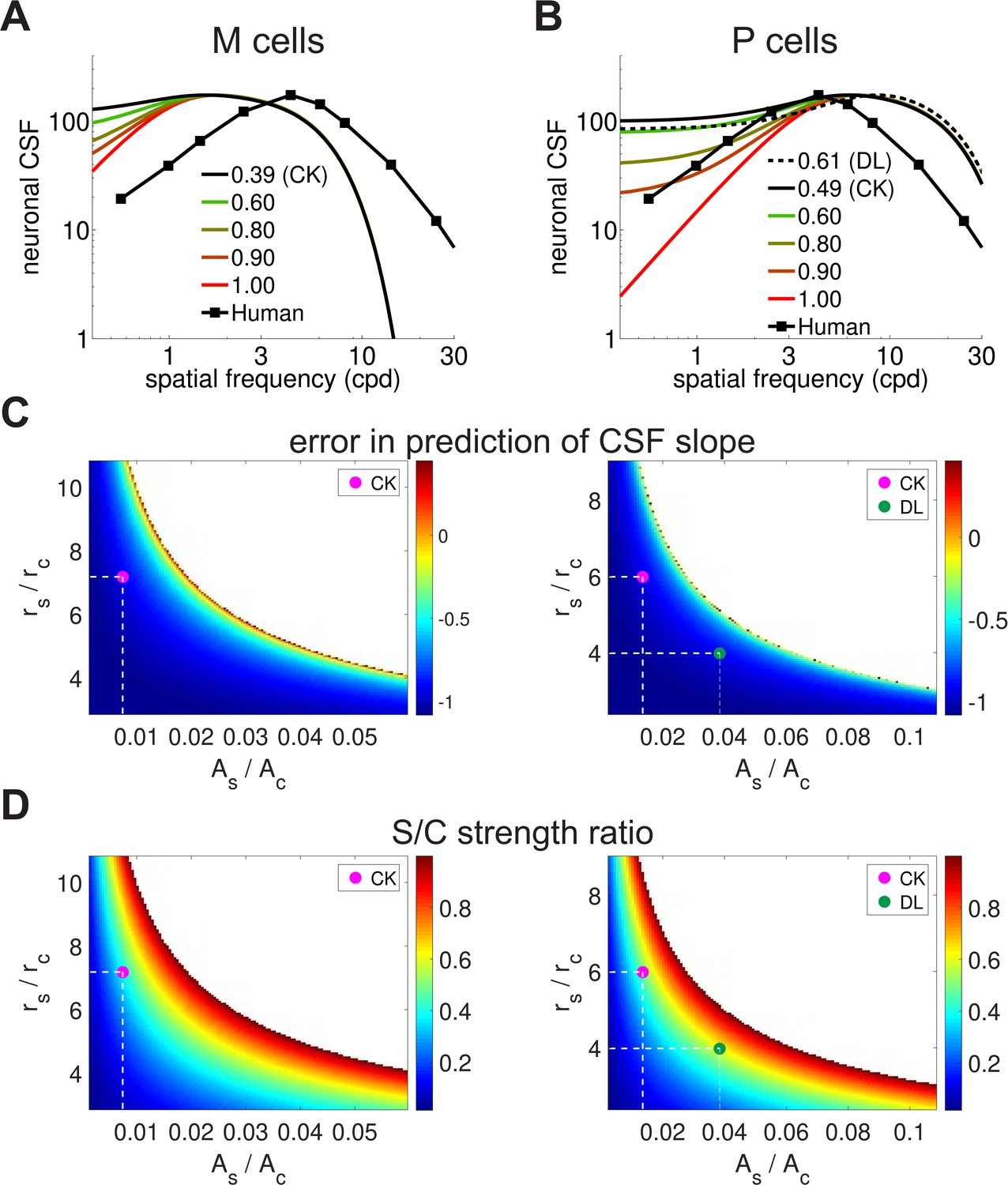
Parametric analysis of the spatial sensitivity of magno- and parvo-cellular neurons.
(A,B) Spatial sensitivity of magno- (A) and parvo-cellular neurons (B) as a function of the ratio between the strengths of their center and surround. The responses of both M and P cells were re-normalized to the maximum of the behavioral CSF (curve labeled "Human", replotted from ) Figure 1A for comparison purposes. 'DL' and 'CK' label the ratios measured experimentally by Derrington and Lennie (1984) and Croner and Kaplan (1995) respectively, from the medians of their reported values. All other parameters were set as described in the Materials and methods section. (C, D) Full parametric analysis of the difference in slope at low spatial frequencies between the human CSF and the spatial sensitivity of difference-of-Gaussians models. Each point in the map shows the slope deviation resulting from a particular ratio between surround and center amplitudes (, horizontal axis) and between radii (, vertical axis) in the models (Equation 3). A value of zero represents perfect matching between the CSF and the receptive fields profile; negative/positive values indicate that the neuronal filter is less/more attenuated than the CSF. Values of the parameters for which the slope could not be computed because the receptive field did not exhibit a band-pass behavior are indicated by white. The magenta and greed dots mark parameters measured experimentally by Croner and Kaplan (1995) and Derrington and Lennie (1984) respectively (dashed lines). (D) Ratio between center/surround excitation and inhibition. A value of 1 indicates that center and surround have the same strength. Legends and symbols are as in C. Comparison of panels C and D shows that a slope similar to that of the human CSF can only be obtained for close balance between excitation and inhibition. These values differ greatly from those measured experimentally (magenta dot).
Figure 2 with 1 supplement

Input transients during measurement of contrast sensitivity.
(A) Temporal modulations in the stimulus. Measurements of contrast sensitivity often change gradually the contrast of the stimulus during the course of the trial. In this case, the stimulus is a static grating. (B) Fixational jitter modulates input signals in a way that depends on the spatial frequency of the stimulus. The same amount of fixational drift yields larger temporal fluctuations with gratings at higher spatial frequencies (vertical arrows). (C) Input power with gratings at 1 and 8 cycles/deg (left panel). Higher spatial frequencies lead to broader temporal distributions (right panel). (D) Total power available at non-zero temporal frequencies with and without fixational drift. In this latter case, temporal modulations are only caused by the temporal contrast envelope of stimulus presentation. Shaded regions represents one standard deviation (see inset). Data represent averages over observers. (E) Temporal sensitivities of modeled retinal ganglion cells. Model parameters are reported in Tables 1 and 2 in Materials and methods.
Figure 2—figure supplement 1
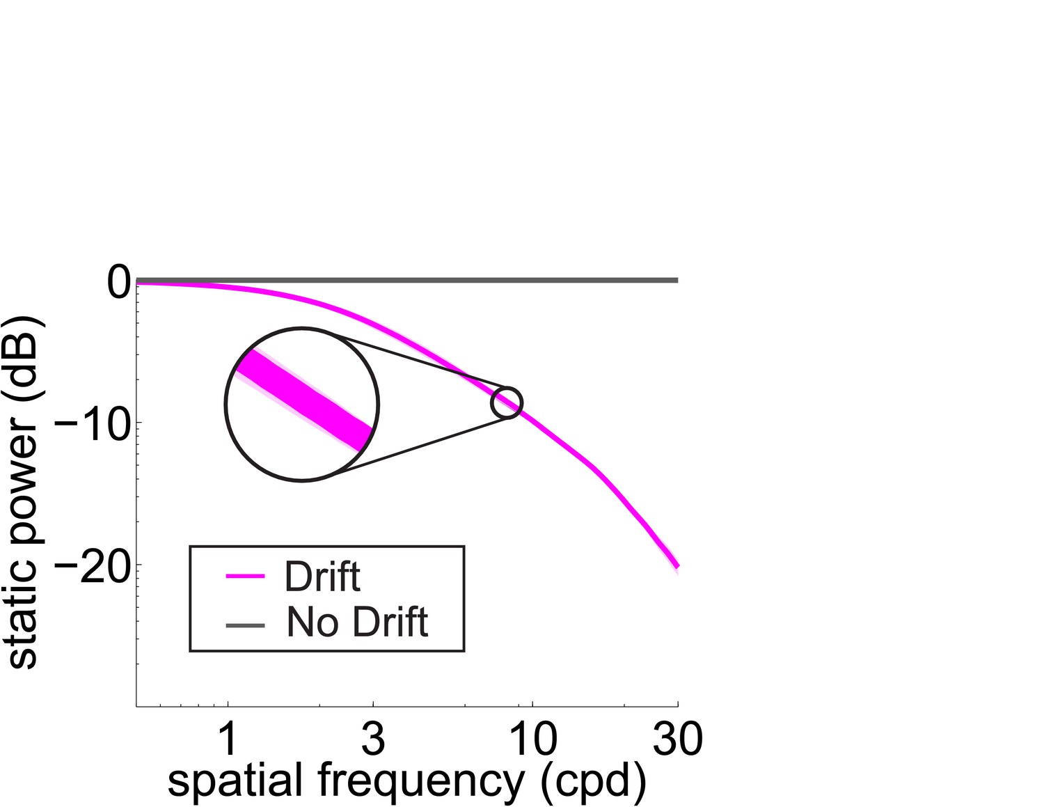
Total power available in the retinal input at 0 Hz (static) with and without fixational drift.
Data represent averages over observers. Symbols are as in Figure 2D.
Figure 3

Influence of fixational drift on contrast sensitivity.
Predicted CSFs in the presence (Drift; solid line) and absence (No Drift; dashed line) of eye movements. Stimuli were stationary gratings. (A) A linear combination of the responses of M and P cells closely matches classical measurements (circles; data from De Valois et al., 1974) only when eye drift occurs. (B–C) CSFs predicted separately from the responses of M (panel B) and P (panel C) cells.
-
Figure 3—source data 1
Source data for Figures 3 and 4 loaded by Source code 1 and 2.
- https://doi.org/10.7554/eLife.40924.009
Figure 4 with 3 supplements
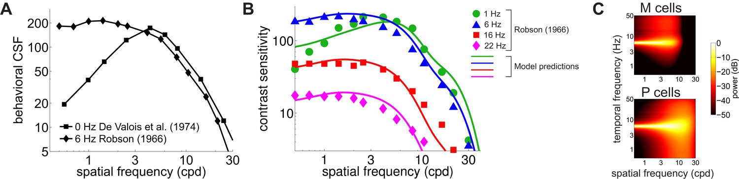
Contributions of fixational drift to contrast sensitivity with temporally modulated gratings.
(A) Human CSFs measured with static (0 Hz; data from De Valois et al., 1974 and sinusoidally modulated (6 Hz; data from Robson, 1966) gratings. (B) Contrast sensitivity functions predicted by our model in the presence of temporally modulated gratings are compared with measurements from Robson (1966). See Figure 4—figure supplement 3 for the separate contributions of M and P cells. (C) Power spectra of the response of modeled retinal ganglion cells during viewing of gratings temporally modulated at 6 Hz. Each point in the map represents the amount of power at a given temporal frequency resulting from translating the modeled receptive fields over a grating at the corresponding spatial frequency following the recorded eye drift trajectories.
Figure 4—figure supplement 1
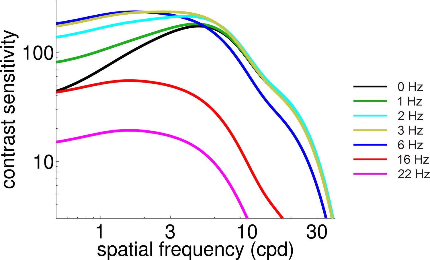
Predicted CSF during normal viewing of temporally modulated gratings.
With respect to Figure 4B, this figure shows a finer sampling of temporal frequencies.
Figure 4—figure supplement 2
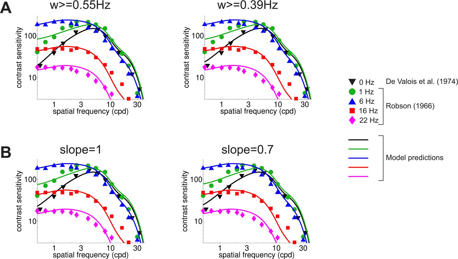
Robustness of the model to the specific implementation of the reduction in sensitivity at low temporal frequencies.
(A) Predicted CSF for two different temporal frequency thresholds. Results in the main text were obtained by discarding temporal power below 0.63 Hz. Results vary little when this threshold is lowered to 0.55 Hz (left panel) or 0.39 Hz (right panel). (B) Predicted CSF when the temporal sensitivity of P cells below 2 Hz was modeled as a power law and power was integrated across all temporal frequencies (no low-frequency threshold). Results are robust with respect to the slope of the power law (1 and 0.7 in the left and right panel, respectively) and virtually identical to those obtained with different integration ranges (cfg. panel (A)).
Figure 4—figure supplement 3
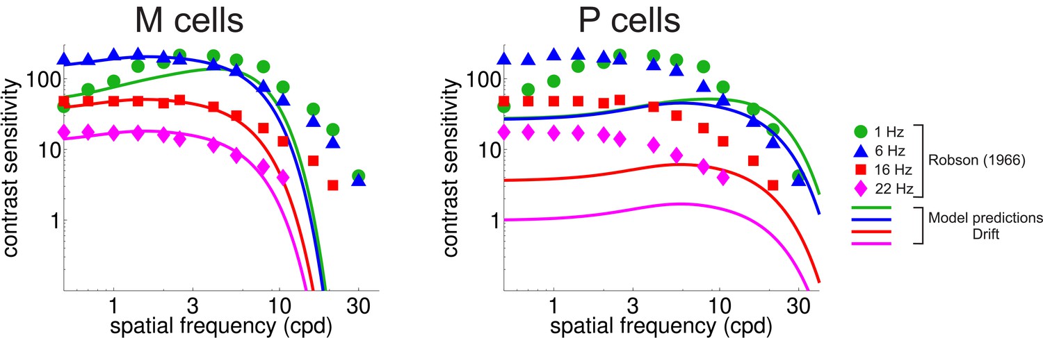
CSF predicted separately from the responses of M and P cells.
Legends and symbols are as in Figure 4B.
Figure 5 with 1 supplement
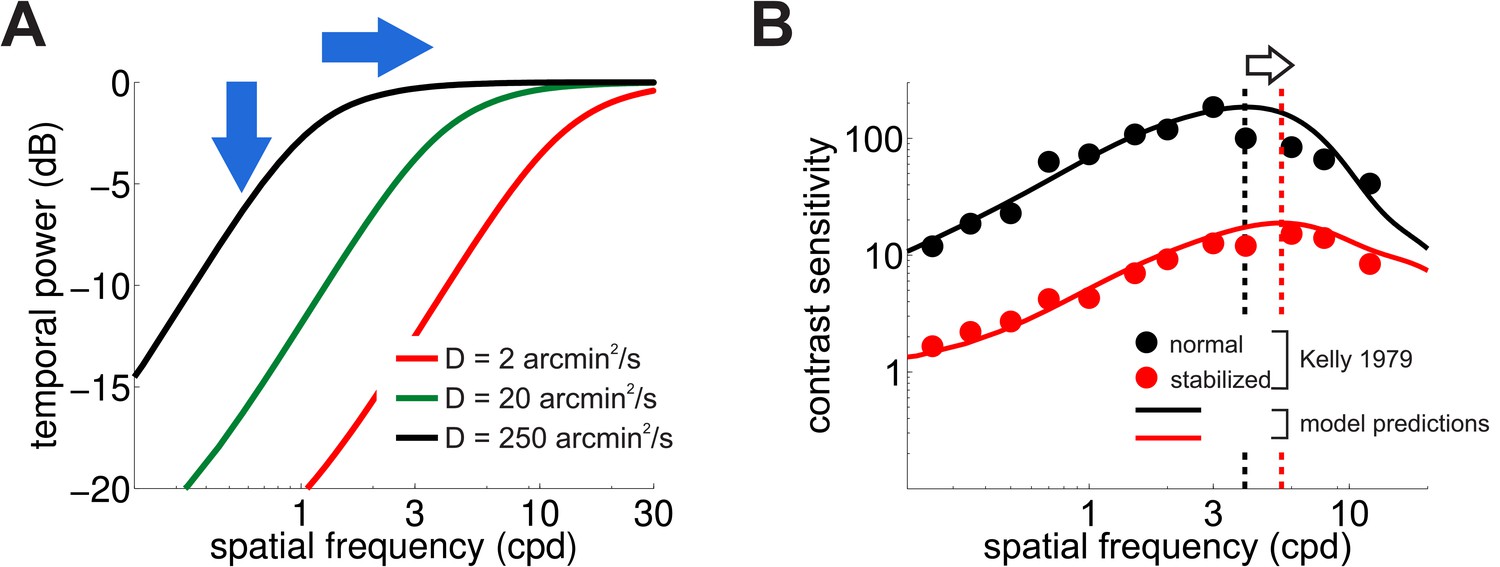
Consequences of retinal stabilization.
(A) Spatial spectral density of the luminance modulations resulting from a Brownian model of retinal image motion with different diffusion constants. Lowering both attenuates the power available at each spatial frequency (vertical arrow) and shifts the distribution to higher spatial frequencies (horizontal arrow). (B) Predicted contrast sensitivity under retinal stabilization. Sensitivity is reduced and shifted to higher spatial frequencies. Dashed vertical lines mark the maxima of the two curves (color coded according to their in panel A). Results quantitatively match classical experimental data from Kelly (1979). CSFs predicted separately from the responses of M and P neurons are shown in Figure 5—figure supplement 1.
-
Figure 5—source data 1
Source data loaded by Source code 3
- https://doi.org/10.7554/eLife.40924.015
Figure 5—figure supplement 1
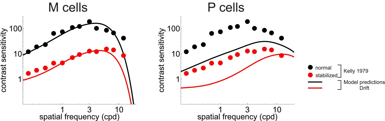
CSF predicted separately from the responses of M and P cells.
Legends and symbols are as Figure 5B, respectively.
Tables
Table 1
Parameters used in Equation 3 to model the spatial kernels of magno- (upper row) and parvo-cellular (bottom row) neurons.
Data are from Croner and Kaplan (1995).
| M cells | 0.10 | 148 | 0.72 | 1.1 |
|---|---|---|---|---|
| P cells | 0.03 | 353.2 | 0.18 | 4.4 |
Table 2
Parameters used in Equation 4 to model the temporal kernels of magno- (upper row) and parvo-cellular (bottom row) neurons.
Data are from Benardete and Kaplan (1997a); Benardete and Kaplan (1999).
| M cells | 30 | 499.77 | 2 | 1 | 1.1 | 2.23 |
|---|---|---|---|---|---|---|
| P cells | 38 | 67.59 | 3.5 | 0.69 | 1.27 | 29.36 |
Additional files
-
Source code 1
Source Matlab code to generate Figures 3A–C in the manuscript.
- https://doi.org/10.7554/eLife.40924.017
-
Source code 2
Source Matlab code to generate Figures 4B in the manuscript.
- https://doi.org/10.7554/eLife.40924.018
-
Source code 3
Source Matlab code to generate Figures 5B in the manuscript.
- https://doi.org/10.7554/eLife.40924.019
-
Transparent reporting form
- https://doi.org/10.7554/eLife.40924.020
Download links
A two-part list of links to download the article, or parts of the article, in various formats.
Downloads (link to download the article as PDF)
Open citations (links to open the citations from this article in various online reference manager services)
Cite this article (links to download the citations from this article in formats compatible with various reference manager tools)
Contrast sensitivity reveals an oculomotor strategy for temporally encoding space
eLife 8:e40924.
https://doi.org/10.7554/eLife.40924


