Crystal structure of a natural light-gated anion channelrhodopsin
Figures
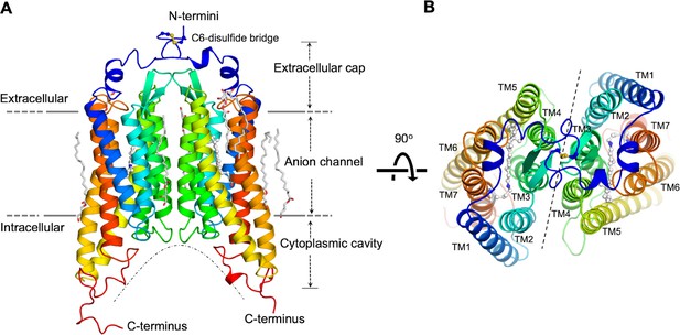
Overall structure of the GtACR1 homodimer.
Side (A), and top (B) views. Each GtACR1 protomer is depicted in cartoon with the N-termini in blue and the C-termini in red. Retinal prosthetic groups (stick-balls) are embedded in the 7TMs. An intermolecular disulfide bridge is formed by C6 (yellow sticks). Resolved monoolein lipids are shown as sticks.
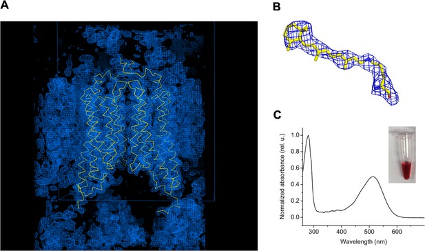
Structural determination of GtACR1.
(A) Electron density map (2fo-fc) contoured at 1.0 σ (blue meshes) in a unit cell. The structure of GtACR1 is displayed as yellow ribbons. (B) Composite omit map (blue mesh) of all-trans-retinal bound with Schiff base K238 contoured at 2.0 σ. The map was calculated by Phenix (Adams et al., 2010). The retinal prosthetic group is drawn as yellow sticks. (C) The absorption spectrum of the purified red-colored GtACR1 protein (inset) showing absorption maximum at 515 nm.
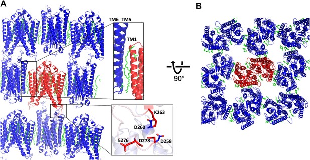
Crystal packing of the GtACR1 structure.
Side (A) and top (B) views. TM1 from one GtACR1 dimer (cartoon in red) interacts with TM5-6 from the adjacent molecule (cartoon in blue) in anti-parallel orientations. Dimer-dimer interaction is mediated by two monoolein lipid molecules (green sticks) on the lateral interface. The 3rd dimension of the lattice is established primarily by contacts between the carboxyl-terminal loops of adjacent molecules. Interactions are highlighted in the magnified views (rectangles).
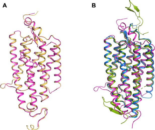
Conserved 7-TM conformation of GtACR1.
(A) Cartoon representation of the two protomers from a GtACR1 homodimer superimposed using secondary structure matching (SSM) by COOT. The r.m.s.d value between protomer A (magenta) and protomer B (yellow) is 0.18 Å. (B) the structure of GtACR1 protomer A (magenta) was superimposed on the structures of C1C2 (green) and the protomer A of CrChR2 (blue) using SSM, showing r.m.s.d. values of ~0.9 Å. Retinal molecules are depicted as sticks.
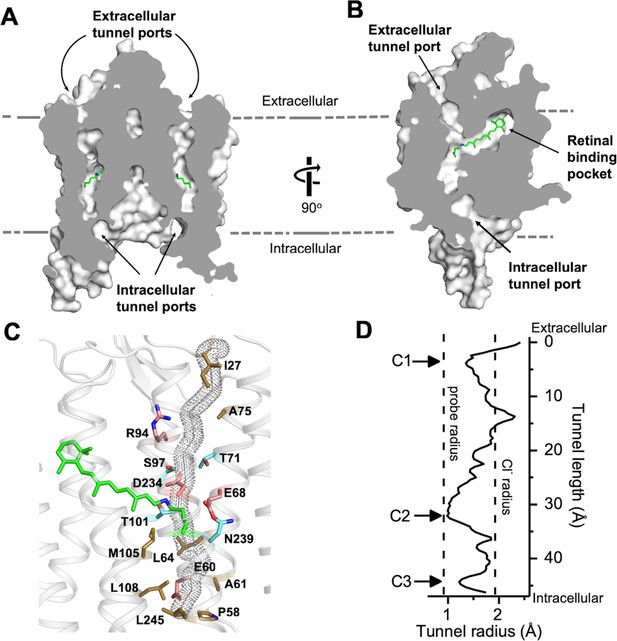
The dark state tunnel of GtACR1.
(A) A cross-section view of the GtACR1 dimer showing two continuous intramolecular tunnels traversing from extracellular ports to the cytoplasmic cavity; retinal (green). (B) A cross-section view of a GtACR1 protomer showing the conformation of the transmembrane ion tunnel and retinal binding pocket connected at the retinylidene Schiff base position. (C) The tunnel (dots) detected by CAVER with tunnel-lining residues (sticks): charged (red), polar (cyan), and apolar residues (clay). (D) The tunnel profile of GtACR1 detected by CAVER; the arrows indicate three constrictions C1-C3.

The predicted tunnel path of GtACR1.
(A) and C1C2 (B) The tunnel paths (dark dots) are predicted by CAVER (probe radius 0.9 Å). Retinal molecules are depicted as green sticks.
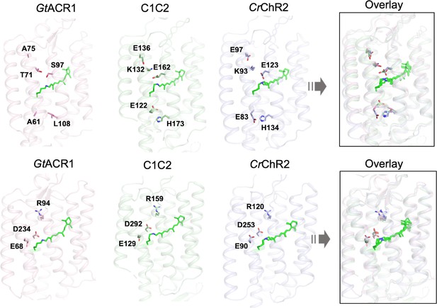
Comparison of selected tunnel-lining residues in GtACR1 with their counterparts in C1C2 and CrChR2.
The five residues in the GtACR1 tunnel that are different from those in C1C2 and CrChR2 are shown on top, and the three highly-conserved tunnel-lining residues in these molecules are shown at bottom. The rightmost panels show overlays of the three structures.
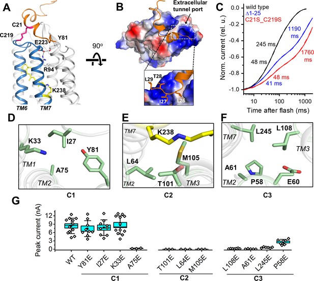
Features of the ion pathway of GtACR1.
(A) The N-terminal extracellular loop (orange) immobilized by an intracellular C21-C219 disulfide bridge (red) to the TM6-7 loop (blue); an H-bond network (black dashed lines) formed by residues (sticks) near the extracellular port. (B) The hydrophobic segment (orange) blocks the extracellular port rendered by the electrostatic potential surface. Rectangle: closer (rotated) view of the peptide cap conformation. (C) Decay kinetics of laser flash-evoked photocurrents by the wild-type GtACR1 and indicated mutants. (D–F) The structure of the three constrictions: C1 (D), C2 (E), and C3 (F). (G) Peak photocurrents generated by Glu substitutions of the constriction residues in response to a 1 s light pulse (515 nm, 7.7 mW mm−2) with 131 mM Cl- in the pipette and 6 mM Cl- in the bath. The black squares, mean; line, median; box, SE; whiskers, SD; empty diamonds, raw data recorded from individual cells.
-
Figure 3—source data 1
Numerical data for the current amplitude values measured in individual cells are shown in Figure 3G.
- https://doi.org/10.7554/eLife.41741.020
-
Figure 3—source data 2
Numerical data for the reversal potential values measured in individual cells are shown in Figure 3—figure supplements 4 and 6.
- https://doi.org/10.7554/eLife.41741.021
-
Figure 3—source data 3
Numerical data for the reversal potential values measured in individual cells are shown in Figure 3—figure supplement 9A.
- https://doi.org/10.7554/eLife.41741.022
-
Figure 3—source data 4
Numerical data for the reversal potential values measured in individual cells are shown in Figure 3—figure supplement 9B.
- https://doi.org/10.7554/eLife.41741.023
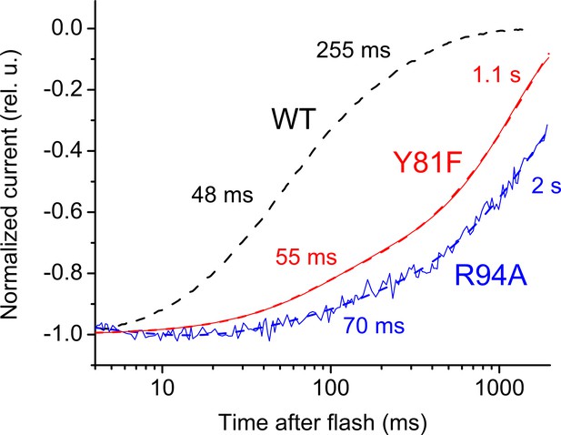
Laser flash-evoked photocurrents generated by the GtACR1_Y81F and R94A mutants, as compared to the wild-type.
Thin solid lines are recorded traces, and thick dashed lines are multiexponential fits. The numbers are the time constants of individual decay phases.
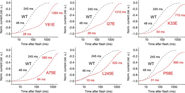
Laser flash-evoked photocurrents generated by the mutants of the C1 and C3 residues.
Thin solid lines are recorded traces, and thick dashed lines are multiexponential fits. The numbers are the time constants of individual decay phases.
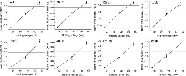
The current-voltage relationships of the the mutants of the C1 and C3 residues measured under a Cl- gradient.
The data points are mean normalized values measured in 5–8 cells (the exact numbers for each mutant are in Table 2), approximated with a B-spline function; the error bars show the sem. For more details see Materials and methods.

The reversal potentials in the mutants of the C1 and C3 residues determined under a Cl- gradient.
The values obtained in individual cells are shown as empty diamonds; the box shows the sem, the whiskers, the sd. The results of Kruskal–Wallis ANOVA are in Table 2.

The current-voltage relationships of the mutants of Q46 and positively charged residues measured under a Cl- gradient.
The data points are mean normalized values measured in 7–13 cells (the exact numbers for each mutant are in Table 3), approximated with a B-spline function; the error bars are the sem. For more details see Materials and methods.
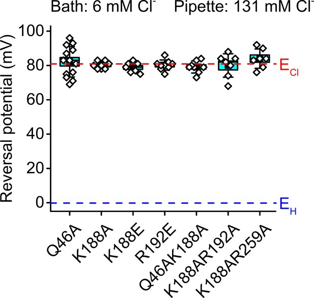
The reversal potentials in the mutants of Q46 and positively charged residues determined under a Cl- gradient.
The values obtained in individual cells are shown as empty diamonds; the box shows the sem, the whiskers, the sd. The results of Kruskal–Wallis ANOVA are in Table 2.
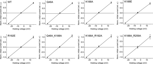
The current-voltage relationships of the mutants of Q46 and positively charged residues measured under a H+ gradient.
The data points are mean normalized values measured in 6–8 cells (the exact numbers for each mutant are in Table 3), approximated with a B-spline function; the error bars are the sem. For more details see Materials and methods.
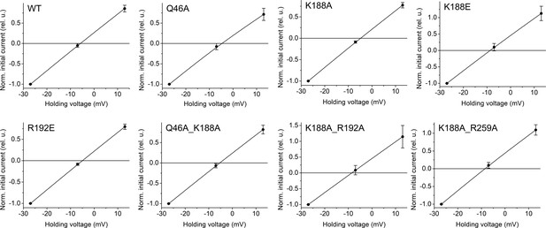
The current–voltage relationships of the mutants of Q46 and positively charged residues measured under a Na+ gradient.
The data points are mean normalized values measured in 6–11 cells (the exact numbers for each mutant are in Table 4), approximated with a B-spline function; the error bars are the sem. For more details see Materials and methods.
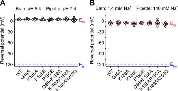
The reversal potentials in the mutants of Q46 and positively charged residues determined under H+ and Na+ gradients.
The values obtained in individual cells are shown as empty diamonds; the box shows the sem, the whiskers, the sd. The results of Kruskal–Wallis ANOVA are in Table 3 and 4.
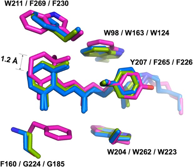
The retinal conformation.
The structure of GtACR1 (magenta) is superimposed with C1C2 (green) and CrChR2 (blue) using SSM. The presence of F160 in GtACR1 (G224/G185 in C1C2/CrChR2, respectively) pushes the β-ionone ring of the all-trans retinal towards the extracellular side by 1.2 Å as measured between the C16 atoms of GtACR1 and CrChR2.

The action spectra of photocurrents generated by the F160G mutant as compared with wild-type GtACR1.
The data points are mean values of 4–6 individual scans. For more detail see Materials and methods.
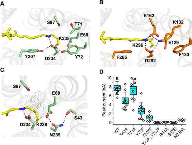
Conformation of the Schiff base region of GtACR1.
(A–B) Structural comparison shows different H-bond networks (dashed lines) in GtACR1 (A) and C1C2 (B). (C) the H-bond network in the ENS triad of GtACR1. The tunnel (black dots) assessed by CAVER. (D) Peak photocurrents generated by the wild-type GtACR1 and indicated mutants in response to laser flash excitation. The black squares, mean; line, median; box, SE; whiskers, SD; empty diamonds, raw data recorded from individual cells.
-
Figure 5—source data 1
Numerical data for the current amplitude values measured in individual cells are shown in Figure 5D.
- https://doi.org/10.7554/eLife.41741.034

The action spectra of photocurrents generated by the Y72F and Y207F mutants, as compared to the wild type.
The data points are mean values of 4–6 individual scans. For more detail see Materials and methods.
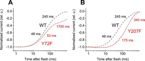
Laser flash-evoked photocurrents generated by the Y72F and Y207F mutants, as compared to the wild type.
Thin solid lines are recorded traces, and thick dashed lines are multiexponential fits. The numbers are the time constants of individual decay phases.

Laser flash-evoked photocurrents generated by.
(A) the S43A and N239A mutants, as compared to the wild type; (B) the D234N, N239A and D234N_N239A_ mutants, as compared to the wild type. Thin solid lines are recorded traces, and thick dashed lines are multiexponential fits. The numbers are the time constants of individual decay phases.
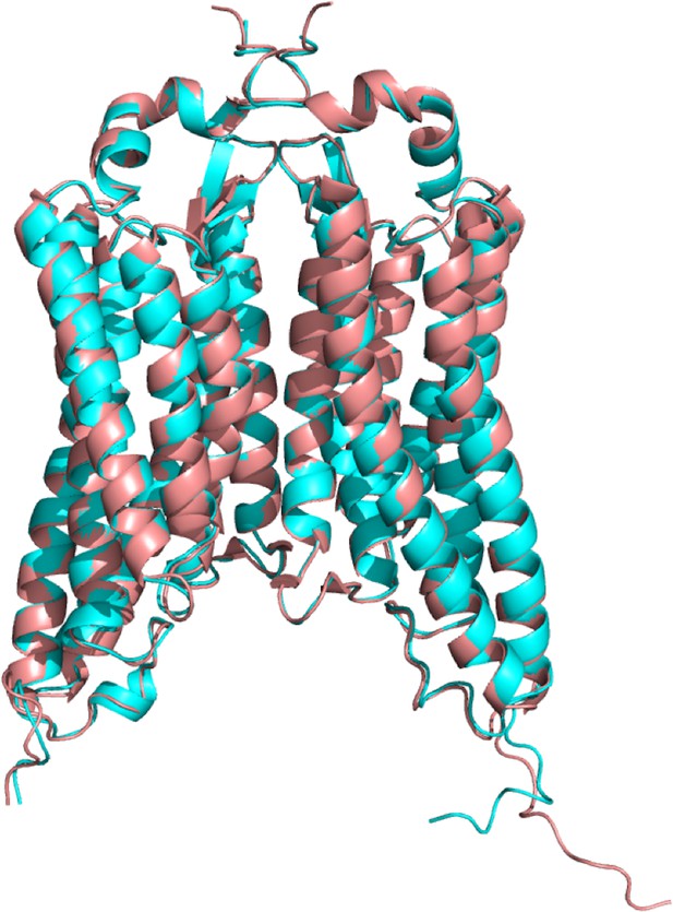
Superposition of two independently obtained GtACR1 structures.
Overview of the GtACR1 structure (PDB code: 6EDQ) colored in cyan superimposed on the structure of GtACR1 reported by Kim et al., 2018 (PDB code: 6CSM) in light pink.
The RMSD value between these two structures is ~0.4 Å.
Tables
Crystallographic data and refinement statistics of the GtACR1 structure
https://doi.org/10.7554/eLife.41741.006| PDB ID | 6EDQ |
|---|---|
| Space group | P21212 |
| a, b, c (Å) | 77.79, 149.55, 62.41 |
| α, β. γ (°) | 90, 90, 90 |
| Beamline | SLS-X06SA |
| Wavelength (Å) | 1.0 |
| Resolution (Å) | 47.91–2.9 (2.98–2.9) |
| Rmeas | 0.39 (2.65) |
| I /σ (I) | 4.54 (0.97) |
| Completeness (%) | 99.8 (100) |
| Multiplicity | 6.89 (6.57) |
| CC1/2 (%) | 99 (32) |
| Refinement | |
| Resolution (Å) | 47.91–2.90 (3.08-2.90) |
| No. of unique reflections | 16711(2732) |
| Rwork/Rfree | 0.23/0.27 |
| R.m.s. deviations | |
| Bond lengths (Å) | 0.005 |
| Bond angles (°) | 0.892 |
| B-factor | |
| Proteins | 63.8 |
| Ligands | 80.1 |
| H2O | 51.0 |
| Ramachandran Plot | |
| Favored (%) | 97.56 |
| Allowed (%) | 2.44 |
| MolProbity Clash score | 9.39 |
-
*Data processing statistics are reported with Friedel pairs merged. Values in parentheses are for the highest resolution shell.
The output of Kriskal-Wallis ANOVA analysis of the results shown in Figure 3—figure supplements 4 and 6
https://doi.org/10.7554/eLife.41741.024| X-Function | Kruskal-Wallis ANOVA | |||||||||||
|---|---|---|---|---|---|---|---|---|---|---|---|---|
| Data filter | No | |||||||||||
| Variant | Data | Range (number of cells) | ||||||||||
| WT | [DataAsp]Sheet1!WT | [1*:10*] | ||||||||||
| Y81E | [DataAsp]Sheet1!Y81E | [1*:7*] | ||||||||||
| I27E | [DataAsp]Sheet1!I27E | [1*:7*] | ||||||||||
| K33E | [DataAsp]Sheet1!K33E | [1*:8*] | ||||||||||
| L108E | [DataAsp]Sheet1!L108E | [1*:7*] | ||||||||||
| A61E | [DataAsp]Sheet1!A61E | [1*:5*] | ||||||||||
| L245E | [DataAsp]Sheet1!L245E | [1*:8*] | ||||||||||
| P58E | [DataAsp]Sheet1!P58E | [1*:7*] | ||||||||||
| Q46A | [DataAsp]Sheet1!Q46A | [1*:13*] | ||||||||||
| K188A | [DataAsp]Sheet1!K188A | [1*:8*] | ||||||||||
| K188E | [DataAsp]Sheet1!K188E | [1*:7*] | ||||||||||
| R192E | [DataAsp]Sheet1!R192E | [1*:9*] | ||||||||||
| Q46AK188A | [DataAsp]Sheet1!Q46AK188A | [1*:8*] | ||||||||||
| K188AR192A | [DataAsp]Sheet1!K188AR192A | [1*:7*] | ||||||||||
| K188AR259A | [DataAsp]Sheet1!K188AR259A | [1*:7*] | ||||||||||
| Variant | N | Min | Q1 | Median | Q3 | Max | ||||||
| WT | 10 | 61 | 70 | 75.5 | 90.25 | 93 | ||||||
| Y81E | 7 | 71 | 73 | 77 | 85 | 85 | ||||||
| I27E | 7 | 75 | 77 | 84 | 86 | 86 | ||||||
| K33E | 8 | 70 | 73.75 | 80 | 85.75 | 87 | ||||||
| L108E | 7 | 69 | 72 | 75 | 76 | 82 | ||||||
| A61E | 5 | 69 | 71 | 74 | 80 | 80 | ||||||
| L245E | 8 | 71 | 73.25 | 75.5 | 85 | 91 | ||||||
| P58E | 7 | 63 | 70 | 75 | 84 | 89 | ||||||
| Q46A | 13 | 69 | 74 | 83 | 90.5 | 96 | ||||||
| K188A | 8 | 78 | 78 | 80 | 82.5 | 83 | ||||||
| K188E | 7 | 75 | 76 | 79 | 81 | 83 | ||||||
| R192E | 9 | 75 | 78.5 | 80 | 81.5 | 86 | ||||||
| Q46AK188A | 8 | 73 | 76.75 | 79 | 82.25 | 84 | ||||||
| K188AR192A | 7 | 68 | 74 | 82 | 84 | 88 | ||||||
| K188AR259A | 7 | 76 | 79 | 84 | 90 | 92 | ||||||
| Variant | N | Mean Rank | Sum Rank | |||||||||
| WT | 10 | 49.55 | 495.5 | |||||||||
| Y81E | 7 | 55.71429 | 390 | |||||||||
| I27E | 7 | 74.28571 | 520 | |||||||||
| K33E | 8 | 62.8125 | 502.5 | |||||||||
| L108E | 7 | 31 | 217 | |||||||||
| A61E | 5 | 36.4 | 182 | |||||||||
| L245E | 8 | 50.125 | 401 | |||||||||
| P58E | 7 | 47.64286 | 333.5 | |||||||||
| Q46A | 13 | 70.30769 | 914 | |||||||||
| K188A | 8 | 65.9375 | 527.5 | |||||||||
| K188E | 7 | 58.14286 | 407 | |||||||||
| R192E | 9 | 66.72222 | 600.5 | |||||||||
| Q46AK188A | 8 | 59.25 | 474 | |||||||||
| K188AR192A | 7 | 66.5 | 465.5 | |||||||||
| K188AR259A | 7 | 84.42857 | 591 | |||||||||
| Chi-Square | DF | Prob > Chi-Square | ||||||||||
| 16.94395 | 14 | 0.25918 | ||||||||||
-
Null Hypothesis: The samples come from the same population.
Alternative Hypothesis: The samples come from different populations.
-
At the 0.05 level, the populations are NOT significantly different.
The output of Kriskal-Wallis ANOVA analysis of the results shown in Figure 3—figure supplement 9A
https://doi.org/10.7554/eLife.41741.025| X-Function | Kruskal-Wallis ANOVA | |||||||||||
|---|---|---|---|---|---|---|---|---|---|---|---|---|
| Data filter | No | |||||||||||
| Variant | Data | Range (number of cells) | ||||||||||
| WT | [DatapH54]Sheet1!WT | [1*:5*] | ||||||||||
| Q46A | [DatapH54]Sheet1!Q46A | [1*:7*] | ||||||||||
| K188A | [DatapH54]Sheet1!K188A | [1*:6*] | ||||||||||
| K188E | [DatapH54]Sheet1!K188E | [1*:8*] | ||||||||||
| R192E | [DatapH54]Sheet1!R192E | [1*:10*] | ||||||||||
| Q46AK188A | [DatapH54]Sheet1!Q46AK188A | [1*:7*] | ||||||||||
| K188AR192A | [DatapH54]Sheet1!K188AR192A | [1*:7*] | ||||||||||
| K188AR259Q | [DatapH54]Sheet1!K188AR259Q | [1*:7*] | ||||||||||
| Variant | N | Min | Q1 | Median | Q3 | Max | ||||||
| WT | 5 | −7.7 | −6.7 | −5.7 | −3.2 | −2.7 | ||||||
| Q46A | 7 | −8.7 | −6.7 | −5.7 | −3.7 | −2.7 | ||||||
| K188A | 6 | −8.7 | −6.45 | −4.7 | −3.95 | −1.7 | ||||||
| K188E | 7 | −9.7 | −4.7 | −3.7 | −2.7 | −2.7 | ||||||
| R192E | 8 | −9.7 | −6.45 | −4.2 | −2.2 | −0.7 | ||||||
| Q46AK188A | 7 | −8.7 | −6.7 | −4.7 | −3.7 | −2.7 | ||||||
| K188AR192A | 7 | −10.7 | −7.7 | −4.7 | −2.7 | −1.7 | ||||||
| K188AR259Q | 7 | −11.7 | −4.7 | −1.7 | 0.3 | 2.3 | ||||||
| Variant | N | Mean Rank | Sum Rank | |||||||||
| WT | 5 | 24.4 | 122 | |||||||||
| Q46A | 7 | 21.71429 | 152 | |||||||||
| K188A | 6 | 24.75 | 148.5 | |||||||||
| K188E | 7 | 30.5 | 213.5 | |||||||||
| R192E | 8 | 28.875 | 231 | |||||||||
| Q46AK188A | 7 | 24.85714 | 174 | |||||||||
| K188AR192A | 7 | 25.21429 | 176.5 | |||||||||
| K188AR259Q | 7 | 38.21429 | 267.5 | |||||||||
| Chi-Square | DF | Prob > Chi-Square | ||||||||||
| 5.33505 | 7 | 0.61915 | ||||||||||
-
Null Hypothesis: The samples come from the same population.
Alternative Hypothesis: The samples come from different populations.
-
At the 0.05 level, the populations are NOT significantly different.
The output of Kriskal-Wallis ANOVA analysis of the results shown in Figure 3—figure supplement 9B
https://doi.org/10.7554/eLife.41741.026| X-Function | Kruskal-Wallis ANOVA | |||||||||||
|---|---|---|---|---|---|---|---|---|---|---|---|---|
| Data filter | No | |||||||||||
| Variant | Data | Range (number of cells) | ||||||||||
| WT | [DataNa1PipNa]Sheet1!WT | [1*:11*] | ||||||||||
| Q46A | [DataNa1PipNa]Sheet1!Q46A | [1*:6*] | ||||||||||
| K188A | [DataNa1PipNa]Sheet1!K188A | [1*:10*] | ||||||||||
| K188E | [DataNa1PipNa]Sheet1!K188E | [1*:6*] | ||||||||||
| R192E | [DataNa1PipNa]Sheet1!R192E | [1*:8*] | ||||||||||
| Q46AK188A | [DataNa1PipNa]Sheet1!Q46AK188A | [1*:7*] | ||||||||||
| K188AR192A | [DataNa1PipNa]Sheet1!K188AR192A | [1*:8*] | ||||||||||
| K188AR259Q | [DataNa1PipNa]Sheet1!K188AR259Q | [1*:10*] | ||||||||||
| Variant | N | Min | Q1 | Median | Q3 | Max | ||||||
| WT | 11 | −11 | -9 | -5 | -3 | 0 | ||||||
| Q46A | 6 | −11 | −8.75 | −2.5 | −0.5 | 1 | ||||||
| K188A | 10 | -9 | −5.5 | -4 | -4 | -2 | ||||||
| K188E | 6 | −14 | −12.5 | −6.5 | −3.75 | -3 | ||||||
| R192E | 8 | -7 | −6.75 | -5 | −2.5 | -2 | ||||||
| Q46AK188A | 7 | -9 | -9 | -5 | -3 | 1 | ||||||
| K188AR192A | 8 | −16 | −13.25 | -4 | −0.5 | 7 | ||||||
| K188AR259Q | 10 | −15 | −9.25 | −7.5 | -5 | -3 | ||||||
| Variant | N | Mean Rank | Sum Rank | |||||||||
| WT | 11 | 34.13636 | 375.5 | |||||||||
| Q46A | 6 | 43.33333 | 260 | |||||||||
| K188A | 10 | 37 | 370 | |||||||||
| K188E | 6 | 26.33333 | 158 | |||||||||
| R192E | 8 | 36.75 | 294 | |||||||||
| Q46AK188A | 7 | 35.5 | 248.5 | |||||||||
| K188AR192A | 8 | 35.3125 | 282.5 | |||||||||
| K188AR259Q | 10 | 22.25 | 222.5 | |||||||||
| Chi-Square | DF | Prob > Chi-Square | ||||||||||
| 6.6454 | 7 | 0.46671 | ||||||||||
-
Null Hypothesis: The samples come from the same population.
Alternative Hypothesis: The samples come from different populations.
-
At the 0.05 level, the populations are NOT significantly different.
| Reagent type (species) or resource | Designation | Source or reference | Identifiers | Additional information |
|---|---|---|---|---|
| Gene (Guillardia theta) | GtACR1 | Synthetic | GenBank: KP171708 | |
| Cell line (Spodoptera frugiperda) | Sf9 | Sigma Aldrich | Sigma Aldrich: 89070101, RRID:CVCL_0549 | |
| Cell line (Homo sapiens) | HEK293 | ATCC | ATCC: CRL-1573, RRID:CVCL_0045 | |
| Recombinant DNA reagent | Cellfectin II Reagent | Thermo Fisher | Cat. No.: 10362100 | https://www.thermofisher.com/order/catalog/product/10362100 |
| Recombinant DNA reagent | ScreenFectA transfection reagent | Waco Chemicals USA | Cat. No.: 299–73203 | http://www.e-reagent.com/uh/Shs.do?now=1544459665328 |
| Recombinant DNA reagent | pFastbac1 | Thermo Fisher | Cat. No.: 10360014 | https://www.thermofisher.com/order/catalog/product/10360014 |
| Recombinant DNA reagent | pcDNA3.1 | Thermo Fisher | Cat. No.: V79020 | https://www.thermofisher.com/order/catalog/product/V79020 |
| Software, algorithm | Pymol | PyMOL Molecular Graphics System, Schrödinger, LLC | RRID:SCR_000305 | http://www.pymol.org/ |
| Software, algorithm | UCSF Chimera | UCSF Resource for Biocomputing, Visualization, and Bioinformatics | RRID: SCR_004097 | http://plato.cgl.ucsf.edu/chimera/ |
| Software, algorithm | PHENIX | PMID: 20124702 | RRID: SCR_014224 | http://www.phenix-online.org/ |
| Software, algorithm | Coot | PMID: 15572765 | RRID: SCR_014222 | http://www.biop.ox.ac.uk/coot/ |
| Software, algorithm | OriginPro 2016 | OriginLab | https://originlab.com | |
| Software, algorithm | pClamp 10 | Molecular Devices | RRID:SCR_011323 | http://www.moleculardevices.com/products/software/pclamp.html |
Additional files
-
Transparent reporting form
- https://doi.org/10.7554/eLife.41741.035


