An integrative genomic analysis of the Longshanks selection experiment for longer limbs in mice
- Friedrich Miescher Laboratory of the Max Planck Society, Germany
- University of Calgary, Canada
- Institute of Science and Technology (IST) Austria, Austria
- Max Planck Institute for Molecular Cell Biology and Genetics, Germany
Figures
Figure 1 with 2 supplements
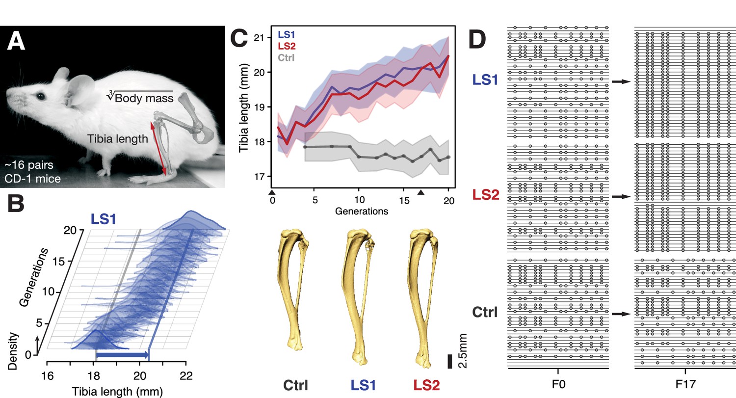
Selection for Longshanks mice produced rapid increase in tibia length.
(A and B) Tibia length varies as a quantitative trait among outbred mice derived from the Hsd:ICR (also known as CD-1) commercial stock. Selective breeding for mice with the longest tibiae relative to body mass within families has produced a strong selection response in tibia length over 20 generations in Longshanks mice (13%, blue arrow, LS1). (C) Both LS1 and LS2 produced replicated rapid increase in tibia length (blue and red; line and shading show mean ±s.d.) compared to random-bred Controls (gray). Arrowheads along the x-axis mark sequenced generations F0 and F17. See Figure 1—figure supplement 1 for body mass data. Lower panel: Representative tibiae from the Ctrl, LS1 and LS2 after 20 generations of selection. (D) Analysis of sequence diversity data (linked variants or haplotypes: lines; variants: dots) may detect signatures of selection, such as selective sweeps (F17 in LS1 and LS2) that result from selection favoring a particular variant (dots), compared to neutral or background patterns (Ctrl). Alternatively, selection may elicit a polygenic response, which may involve minor shifts in allele frequency at many loci and therefore may leave a very different selection signature from the one shown here.
Figure 1—figure supplement 1
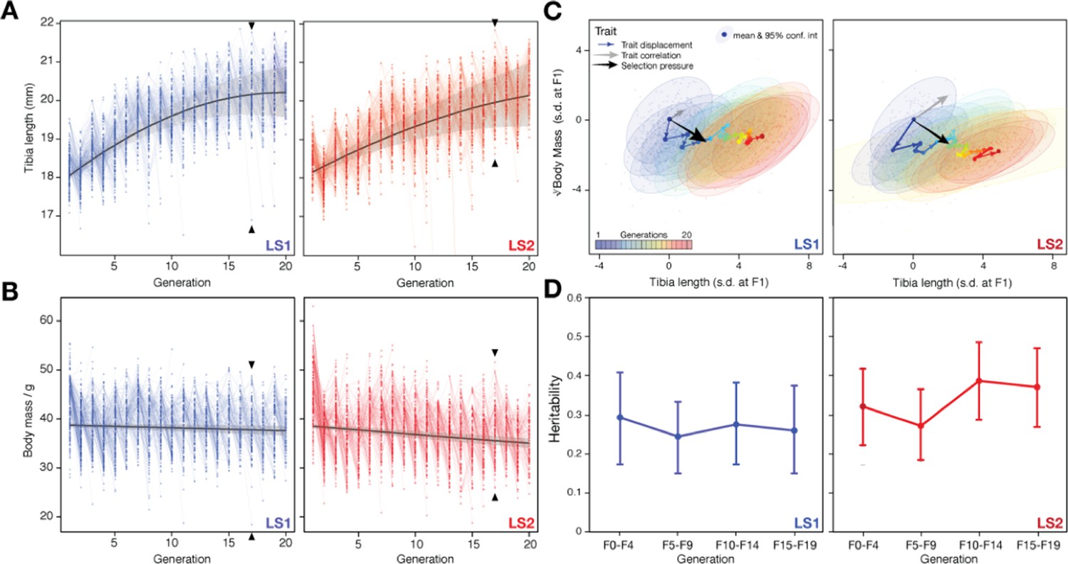
Artificial selection allowed detailed reconstruction of selection parameters.
Rapid response to selection produced mice with progressively longer tibiae (A) and slightly lower body weight (B) within 20 generations. Having complete records throughout the selection experiment makes it possible to reconstruct the selection response for both phenotypes and genotypes in detail. Individuals varied in tibia length in both Longshanks lines (LS1, left; LS2, right). Lines connect parents to their offspring. The actual selection depended on the within-family and within-sex rank order of the tibia length-to-body mass (cube root) ratio (see Marchini et al., 2014 for details). The overall selection response was immediate and rapid for tibia length (A), suggesting a selection response that depended on standing variation among the founders (black lines show the best fitting quadratic function, with shading indicating 95% confidence interval; adjusted R2 = 0.61 for LS1; 0.43 for LS2). Strong selection response led to rapid increase in tibia length. In contrast, there was only minor decrease in body weight over the course of the experiment. (C) Trajectory in selection response shows decoupling of correlation between tibia length and body mass. Despite overall correlation between tibia length and body mass (gray arrow and major axes in confidence envelopes), cumulative trait displacement over the 20 generations (expressed in s. d. units at F1; arrows, dots and 95% confidence envelopes, color-coded according to generation) showed persistent increase in tibia length with only minor change in body mass along the general direction of selection pressure (black arrows from F1; vector length and directions based on logistic regression). This shows that the Longshanks selection experiment was successful in specifically selecting for increased tibia length while keeping relatively unchanged body mass. (D) Despite persistent and strong selection, heritability for the composite trait ( = tibia length in mm; = cube-root body mass in ) (see Simulating selection response: infinitesimal model with linkage in main text) was maintained over 20 generations. Heritability was estimated by a linear mixed “animal model” in which the phenotypic variance was partitioned as VP = fixed effects + VA + VR, where fixed effects were sex, age, and litter size, VA was additive genetic variance, and VR was residual variance. Heritability was estimated as h2 = VA /(VA + VR). Each tested block used the full pedigree but only phenotypic information from individuals within the block. We tested an alternate model for each block using truncated pedigrees wherein the first generation of each block was assumed to be unrelated, but found similar results.
Figure 1—figure supplement 2
Simulating selection on pedigrees.
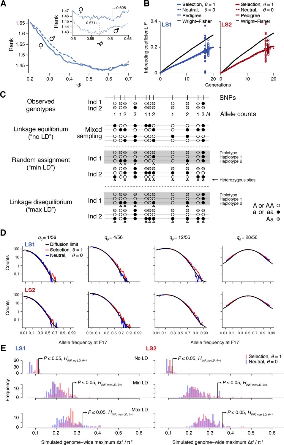
This figure summarizes the results from our analyses to determine parameters used in the simulations. For full detail, see Appendix, section ‘Major considerations in constructing the simulations’. (A) Finding the correct value for the composite trait . In each simulated family, offspring are split by sex and ranked by their composite trait. Due to occasional use of back-up crosses, the average rank of actual breeders is greater than 1. We vary to find the value where actual breeders in the LS lines have the best (lowest) rank. We find = -0.571 to show the best match for males and -0.605 for females. For subsequent analyses we set to be -0.57. (B) Increase in inbreeding over the course of the Longshanks experiment. The lines show the change in identity between two alleles between diploid individuals, , over 20 generations, as calculated from the pedigree (light shade); the average of 50 neutral simulations without selection (dotted line); or the average of 50 simulation replicates with selection intensity at = 0.584 (; thick, dark line). While the trajectories based on pedigree or neutral simulations are indistinguishable, inbreeding increases slightly faster under selection (thick line). The black line shows the increase in identity expected under a Wright–Fisher model with the actual population sizes; under this model, and are close to each other, and to , with equal to the harmonic mean, 24.8. The large dot (with error bar showing the interquartile range among chromosomes) at right show the actual , estimated from the decline in average over 17 generations. Small filled dots show the estimates from each of the 20 chromosomes. Open dots show 40 replicate simulations, made with the same pedigree and the same selection response and sub-sampling from the simulated chromosome according to the actual map length of each of the mouse chromosomes (Cox et al., 2009). The simulation agrees well with the observed genome-wide average. Most of the observed data from chromosomes fall within a range comparable to simulated replicates (compare large dot with open dots), with LD being the likely source of this excess variance. (C) Three different schemes to seed founder haplotypes. We simulate founder haplotypes that are consistent with observed genotypes (shown here as black, white and gray dots as the two homozygous and the heterozygous states) by directly sampling from founder individuals in each LS line. Under the linkage equilibrium scheme, we sample from the list of allele counts at all SNPs. This produces founder haplotypes that carry no linkage disequilibrium (‘no LD'). Under the random assignment scheme, we sample according to each individual (shown as ‘diplotypes' within the box for easy comparison). At heterozygote sites in each individual (arrowheads), we randomly assign the alleles to the two haplotypes. This produces founder haplotypes that show minimal LD that is consistent with the observed genotypes (‘min LD'). Under the ‘max LD' assignment scheme, we also sample according to each individual, except that we consistently assign its haplotypes 1 and 2 with reference (white) and alternate (black) alleles, respectively. This maximizes LD in the founder haplotypes (‘max LD'). (D) Simulated vs. expected allele frequency shifts. The distribution of minor allele frequencies q0 at generation 17 is compared with the distribution expected with no selection (blue) or with selection (red), given a frequency of 1, 4, 12 or 28 minor alleles out of 56 founding alleles. The black line shows the diffusion limit, calculated for scaled time , with estimated to be 51.7 and 48 in LS1 and LS2 respectively, from the rate of increase in , calculated from the pedigree in panel A above. (E) Significance threshold values under varying LD from 100 simulated replicates (blue: no selection; red: observed selection response in the actual experiment, ; see panel C on LD assignment methods). In order to account for non-independence of adjacent windows due to linkage, a distribution of genome-wide maximum ∆z2 was used to determine the significance threshold at each LD level. ∆z2 is the square of arcsine transformed allele frequency difference between F0 and F17; this has an expected variance of 1/2Ne per generation, independent of starting frequency, and ranges from 0 to π2. As seen in previous panels, increasing selection pressure does produce greater shifts in ∆z2 despite using the same pedigree due to a relatively greater proportion of additive genetic variance . However, a far greater impact on ∆z2 is due to changes in LD. This is because weak associations between large numbers of SNP can greatly inflate the variance of ∆z2. Of the three LD levels, ‘max LD' likely produced overly conservative thresholds, whereas ‘min LD' may lead to higher false positives. We have opted conservatively to use maximal LD in our analysis.
Figure 2 with 4 supplements
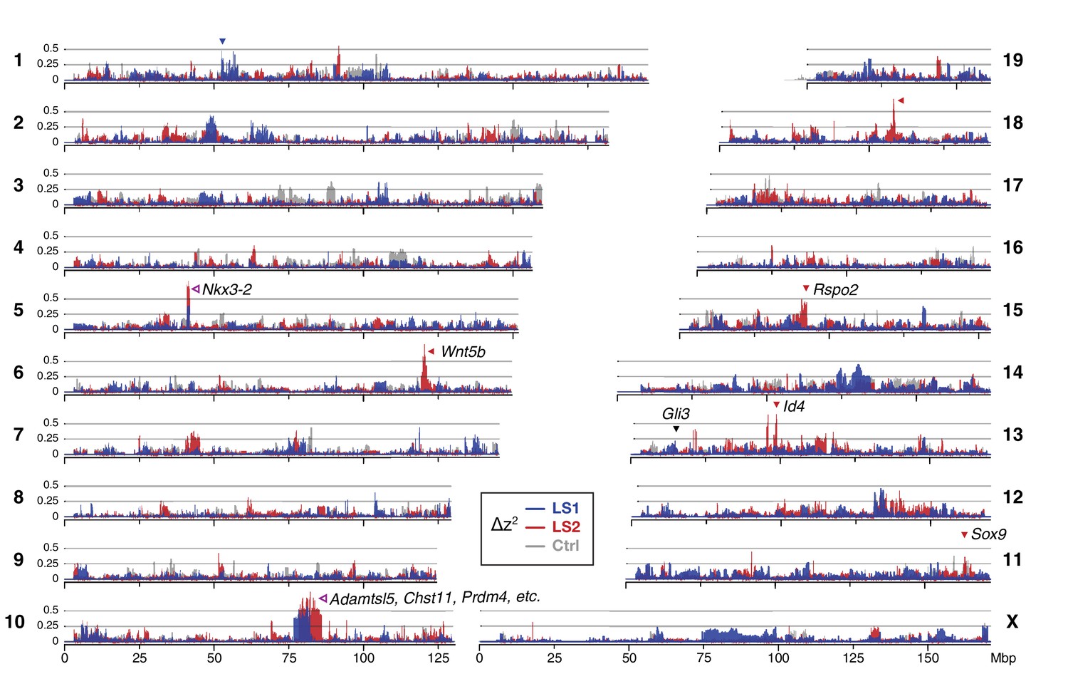
Widespread genomic response to selection for increased tibia length.
Allele frequency shifts between generations F0 and F17 in LS1, LS2 and Ctrl lines are shown as ∆z2 profiles across the genome (plotted here as fraction of its range from 0 to π2). The Ctrl ∆z2 profile (gray) confirmed our expectation from theory and simulation that drift, inbreeding and genetic linkage could combine to generate large ∆z2 shifts even without selection. Nonetheless the LS1 (blue) and LS2 (red) profiles show a greater number of strong and parallel shifts than Ctrl. These selective sweeps provide support for the contribution of discrete loci to selection response (arrowheads, blue: LS1; red: LS2; purple: parallel; see also Figure 1—figure supplement 2E, Figure 2—figure supplement 2, Figure 2—figure supplement 3) beyond a polygenic background, which may explain a majority of the selection response and yet leave little discernible selection signature. Candidate genes are highlighted (Table 1). An additional a priori candidate limb regulator Gli3 is indicated with a black arrowhead.
Figure 2—figure supplement 1

Broad similarity in molecular diversity in the founder populations for the Longshanks lines and the Control line.
(A) Shown are the site frequency spectra from LS1, LS2 and Control lines at F0 (top; folded based on a global minor allele frequency or MAF ≤0.5) and F17 (bottom; unfolded, but tracking the same minor alleles as in F0). Overall the spectra were very similar to each other within each generation. The Control population was mostly intermediate in the decay in the rarer alleles. After 17 generations, the same alleles were generally more spread out, leading to more broadly distributed spectra. There was again little overall difference between the Longshanks and Control lines. (B) Variations between chromosomes (separate same-colored lines) shown in each population and generation. The unfolded site frequency spectrum is shown based on the MAF assigned as in A. There is substantial variation between chromosomes, which shows increased distortions in F17. (C) Allele frequencies between the founder populations were very similar. Joint minor allele frequencies shown as box plots in 2% bands between the Control and LS1 (blue), LS2 (red); or the two LS lines (purple). Outliers were omitted for clarity. The overall trends follow closely the parity line (gray line along the diagonal), except at frequencies very close to 0.5. Similar to the site frequency spectra in panel A, a small number of sites have a MAF above 0.5 (gray box), because of the use of an overall MAF ≤0.5 to determine minor allele status to enable comparisons across lines. Correlations between all pairwise combinations were around 0.93.
Figure 2—figure supplement 2
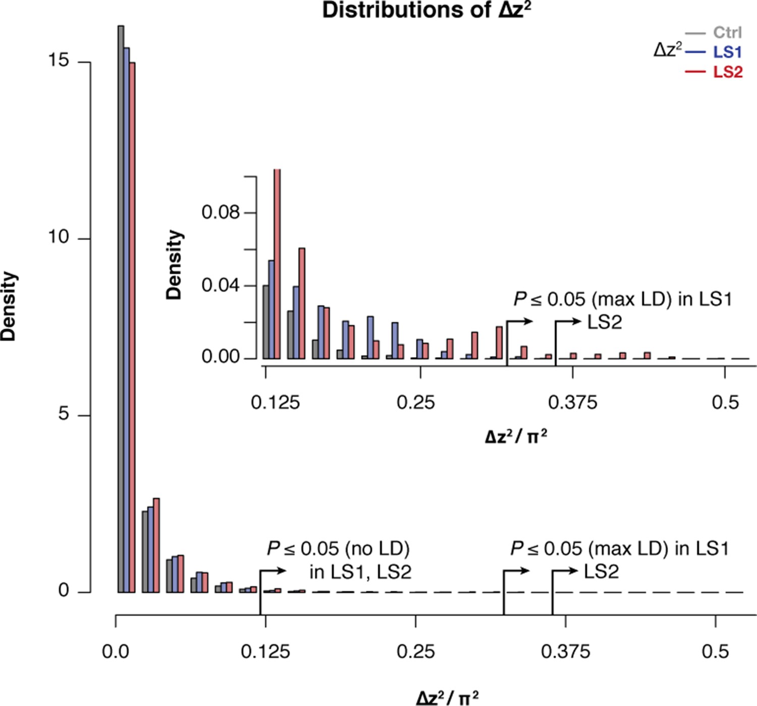
Selected lines showed more extreme values of ∆z2 than the Control line.
Histogram of within-line ∆z2 values in 10 kbp windows across the genome in LS1, LS2, and Control. Overall similarity is high across all three lines, but there was an excess of large ∆z2 value starting from as low as <0.1 π2. This pattern becomes clearly distinct above the threshold value of 0.125, which corresponds to the lenient significance threshold p≤0.05 under HINF, no LD (inset). There was clearly an excess of windows in LS2 above the more stringent p≤0.05 threshold under HINF, max LD. This excess supports discrete loci contributing to selection response in LS2 that give rise to greater distortion of ∆z2 spectra.
Figure 2—figure supplement 3
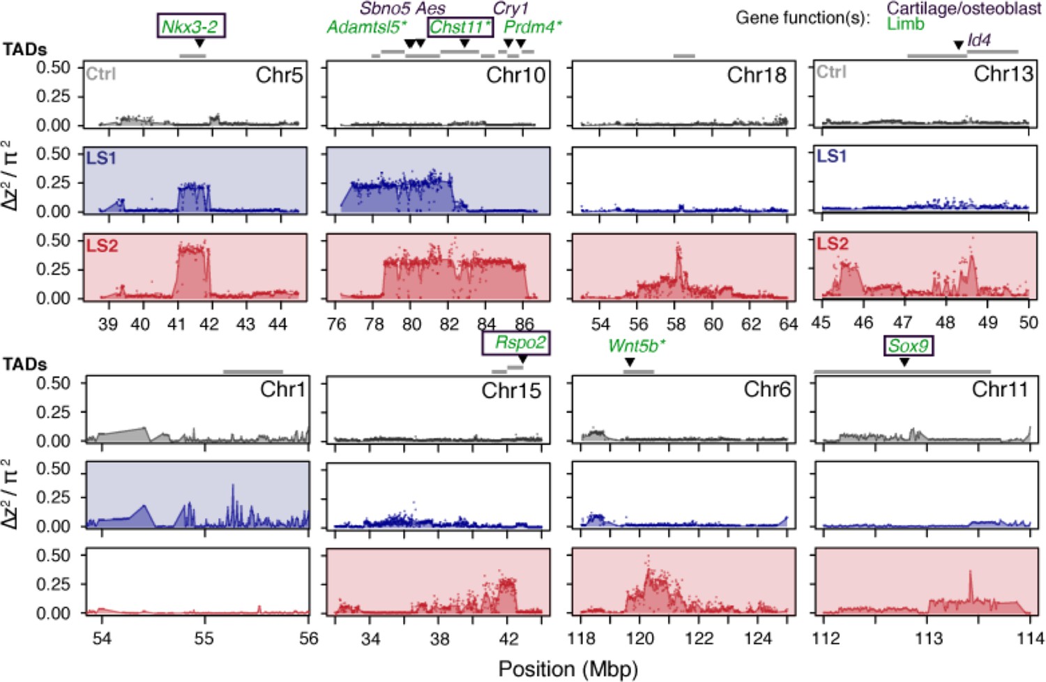
Detailed ∆z2 profiles at the 8 Longshanks significant loci.
For each significant locus, ∆z2 profiles are shown for Ctrl (gray), LS1 (blue) and LS2 (red). Plots are shaded if the locus is significant in a given line. TADs within 250 kbp of the significant signals are shown as gray bars above each locus. Above the TADs are highlighted genes whose knockout phenotypes belong to the following categories: ‘abnormal tibia morphology’, ‘short limb’, ‘short tibia’, ‘abnormal cartilage morphology’, ‘abnormal osteoblast morphology’. The gene symbols are colored according to the gene function(s) in limb development (green), bone development (purple) or both (boxed). Gene symbols marked by asterisks (*) have specifically reported ‘short tibia’ or ‘short limb’ knockout phenotypes. All of the above categories show significant enrichment at the eight loci (number of genes per category: 4–7, nominal p≤0.03, see Appendix, section ‘Enrichment for genes with functional impact on limb development’ for details on the permutation), except ‘abnormal cartilage morphology’, with four genes and a nominal P-value of 0.083. No overlap was found with any gene in these categories from the three significant loci from the Ctrl line.
Figure 2—figure supplement 4

Loci associated with selection response in Longshanks lines show enrichment for limb function likely associated with cis-acting mechanisms.
(A) Gene set enrichment analysis of knock-out phenotypes (KO) showed that selection response (here shown as ∆z2 cut-off values, see Supplementary Methods for details on cut-off values and inclusion criteria) were found among topologically associating domains (TADs) containing limb and tail developmental genes (red solid lines) or genes with limb expression (red dotted lines) in LS lines (top) but not in Ctrl (bottom). Among KO phenotypes, limb defects show the greatest excess out of 28 phenotypic categories (other gray lines, with other extreme categories labeled, the ‘normal’ category is excluded here). Among developmental enhancers for limb, heart, liver and brain tissue, we also observed an association with ∆z2 peaks in LS lines (top) for limb but not in Ctrl lines (bottom). The simulated significance thresholds based on HINF, max LD are also shown for reference (vertical gray lines). The data from the LS lines suggest that enrichment started to increase around the p≤0.5 threshold and remained largely stable at p≤0.05, corresponding to a cut-off of around 0.33 π2. (B) Coding vs. regulatory impact. Frequency of moderate to major coding changes (top panels, amino acid changes, frame-shifts or stop codons), or average conservation score of regulatory sequences immediately flanking SNPs (based on conservation among 60 eutherian mammals; bottom panels) were used as proxies to estimate the functional impact of coding and regulatory mutations, respectively. In LS1, major coding changes became more common at high ∆z2 ranges; however the number of SNPs with potentially major phenotypic consequences did not increase in LS2 and in fact seemed to decrease in Ctrl. In contrast, regulatory changes showed increased conservation associated with greater allele frequency shifts or ∆z2 in all three lines, except that SNPs with large shifts and strong conservation were more abundant in LS1 and LS2. Trend lines are shown with LOESS regression but statistical comparisons were performed using linear regressions.
Figure 3 with 1 supplement
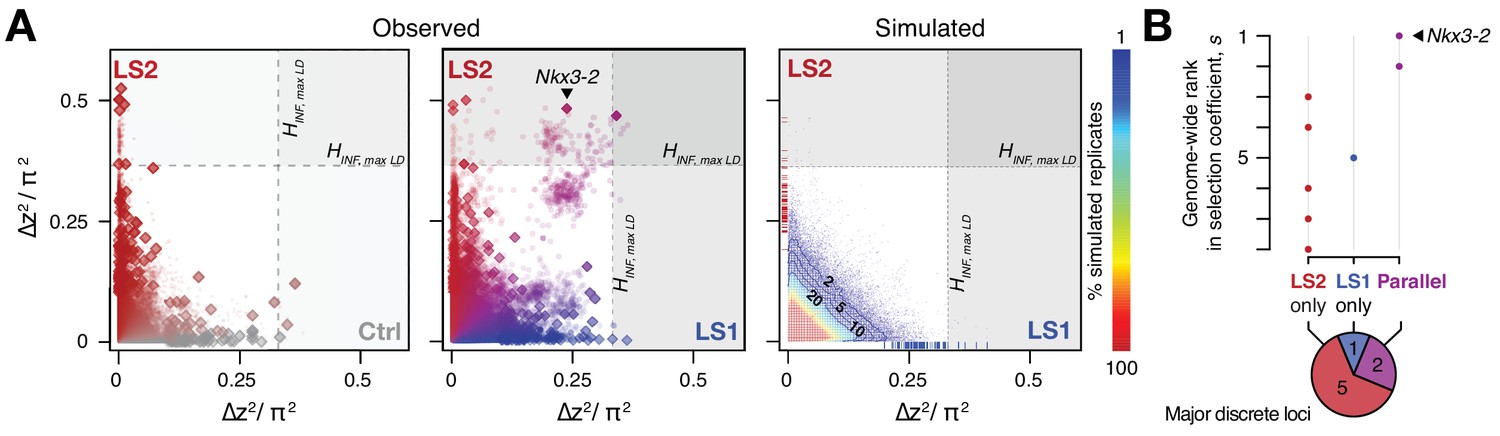
Selection response in the Longshanks lines was largely line-specific, but the strongest signals occurred in parallel.
(A) Allele frequencies showed greater shifts in LS2 (red) than in Ctrl (gray; left panel; diamonds: peak windows; dots: other 10 kbp windows; see Figure 3—figure supplement 1 for Ctrl vs. LS1 and Appendix for details). Changes in the two lines were not correlated with each other. In contrast, there were many more parallel changes in a comparison between LS1 (blue) vs. LS2 (red; middle panel; adjacent windows appear as clusters due to hitchhiking). The overall distribution closely matches simulated results under the infinitesimal model with maximal linkage disequilibrium (HINF, max LD; right heatmap summarizes the percentage seen in 100 simulated replicates), with most of the windows showing little to no shift (red hues near 0; see also Figure 3—figure supplement 1 for an example replicate). Tick marks along the axes show genome-wide maximum ∆z2 shifts in each of 100 replicate simulations in LS1 (x-axis, blue) and LS2 (y-axis, red), from which we derived line-specific thresholds at the p≤0.05 significance level. While the frequency shifts from simulations matched the bulk of the observed data well, no simulation recovered the strong parallel shifts observed between LS1 and LS2 (compare middle to right panel, points along the diagonal). (B) Genome-wide ranking based on estimated selection coefficients s among the candidate discrete loci at p≤0.05 under HINF, max LD. While six out of eight total loci showed significant shifts in only LS1 or LS2, the two loci with the highest selection coefficients were likely selected in parallel in both LS1 and LS2 (also see middle panel in A).
Figure 3—figure supplement 1
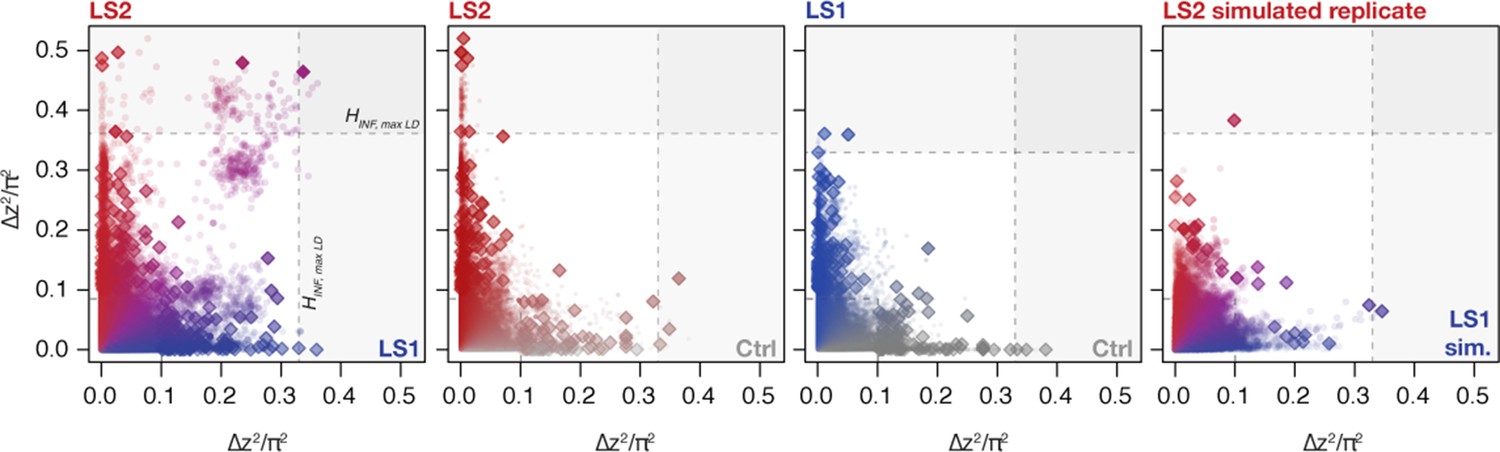
Changes in ∆z2 across lines.
Shown are changes in ∆z2 in individual 10 kbp windows (all windows: circles; peak windows: diamonds). Generally there were no clear differences in ∆z2 along the axes except a slight skew toward higher values in LS2. When taken as a joint LS1–LS2 comparison, however, we observed that many windows show shifts in both LS1 and LS2 (left panel; in purple). In contrast, very few windows show parallelism in Ctrl–LS2 and Ctrl–LS1 comparisons (middle two panels). The right panel shows a single selected simulated replicate (selection pressure ; maximum LD) found to have among the greatest extent of parallel ∆z2 among the replicates. The excess in parallel loci in observed results is clear both among the significant loci at p≤ 0.05 under HINF, max LD and highly significant at the more relaxed HINF, no LD threshold.
Figure 4 with 2 supplements

Strong parallel selection response at the bone maturation repressor Nkx3-2 locus was associated with decreased activity of two enhancers.
(A) ∆z2 in this region of chromosome five showed strong parallel differentiation spanning 1 Mbp in both Longshanks but not in the Control line. This 1 Mbp region contains three genes: Nkx3-2, Rab28 and Bod1l (whose promoter lies outside the TAD boundary, shown as gray boxes). Although an originally rare allele in all lines, this region swept almost to fixation by generation 17 in LS2 (Figure 5—figure supplement 1A). (B) Chromatin profiles [ATAC-Seq, red, (Buenrostro et al., 2013); ENCODE histone modifications, purple] from E14.5 developing limb buds revealed five putative limb enhancers (gray and red shading) in the TAD, three of which contained SNPs showing significant frequency shifts. Chromosome conformation capture assays (4C-Seq) from E14.5 limb buds from the N1, N2 and N3 enhancer viewpoints (bi-directional arrows) showed significant long-range looping between the enhancers and sequences around the Nkx3-2 promoter (heat-map from gray to red showing increasing contacts; Promoters are shown with black arrows and blue vertical shading). (C) Selected alleles at 7 SNPs found within the N1, N2, and N3 enhancers increased ~0.75 in frequency in both LS1 and LS2. Selected alleles at three of these sites are predicted to lead to loss (red inhibition circles) of transcription factor binding sites in the Nkx3-2 pathway (including a SNP in N3 causing loss of two adjoining Nkx3-2 binding sites) and thus reduce enhancer activity in N1 and N3. (D, E) Transient transgenic reporter assays of the N1 and N3 enhancers showed that the F0 alleles drove robust and consistent expression at centers of future cartilage condensation (N1) and broader domains of Nkx3-2 expression (N3) in E12.5 fore- and hind limb buds (FL, HL; ti: tibia). Fractions indicate the number of embryos showing similar lacZ staining out of all transgenic embryos. Substituting the F17 enhancer allele (i.e., replacing three positions each in N1 and N3) led to little observable limb bud expression in both the N1/F17 and N3/F17 embryos, suggesting that selection response for longer tibia involved de-repression of bone maturation through a loss-of-function regulatory allele of Nkx3-2 at this locus. Scale bar: 1 mm for both magnifications.
Figure 4—figure supplement 1
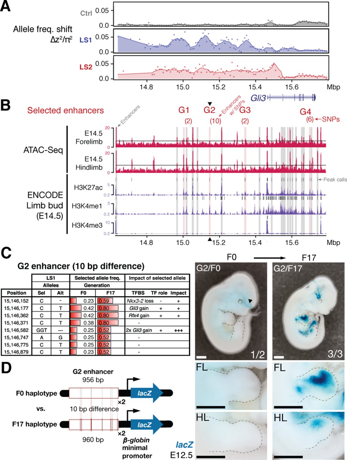
An enhancer in chromosome 13 boosts Gli3 expression during limb bud development.
(A) LS1 showed elevated ∆z2 in the intergenic region containing Gli3. (B) Putative limb enhancers (gray bars) were identified through peaks from ATAC-Seq (top) and histone modifications (bottom tracks, data from ENCODE project). Four of the enhancers contain mutations (in parentheses) with significant allele frequency shifts between F0 and F17 in LS1 (red shading). One of the enhancers located close to the peak ∆z2 signal (G2, arrowhead) containing 10 bp differences was chosen for transgenic reporter assay. (C) Analysis of individual mutations showed an average increase of 0.33 in allele frequency, with six mutated positions affecting predicted binding of transcription factors in the Gli3 pathway (including three additional copies of Gli3 binding sites), all of which are predicted to boost the G2 enhancer activity. (D) The F17 G2 enhancer variants together drove robust and consistent lacZ reporter gene expression at E12.5, recapitulating Gli3 expression in the developing fore- and hind limb buds (right; see also Figure 4—figure supplement 2). Substitution of 10 positions (F0 haplotype) led to little observable expression in the limb buds (left). These G2 enhancer gain-of-function mutations (contrasting the major allele between F0 and F17) may confer an advantage under selection for increased tibia length. Scale bars: 1 mm for both magnifications.
Figure 4—figure supplement 2
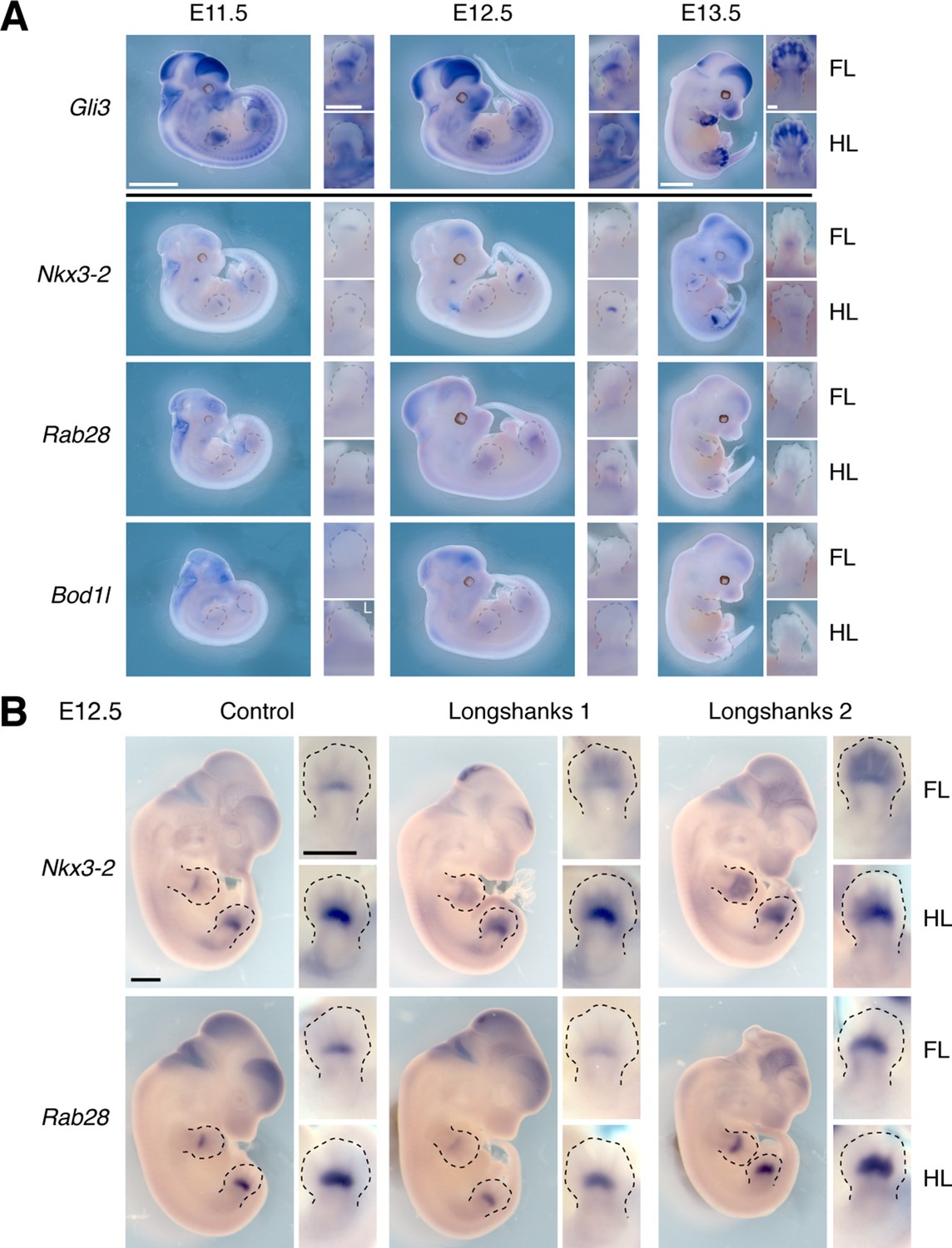
Gene expression patterns at the Gli3 and Nkx3-2 candidate intervals.
(A) Gli3 expression was determined using in situ hybridization. Gli3 was robustly expressed during limb development in both developing fore- and hindlimb buds, especially in the autopod (hand/foot plate). Lower panels show expression of Nkx3-2 and its neighboring genes Rab28 and Bod1l. The stronger expression of Nkx3-2 in the developing limb buds as well as the known role of Nkx3-2 in bone maturation (Sivakamasundari et al., 2012) strongly argues for Nkx3-2 being the gene underlying the selection response at the chromosome 5 locus. Scale bars: 1 mm for whole-mounts; 0.5 mm for limb buds. FL, forelimb; HL, hind limb; unless otherwise indicated by ‘L’, all images were taken from the right side. (B) We collected E12.5 embryos from each line and performed in situ hybridization to determine the sites and level of expression of Nkx3-2 and Rab28 in the Longshanks (right columns) and Control (left column) lines. Both genes are expressed in similar sites overall and specifically in the developing fore- and hind limb buds in the region of the presumptive zeugopods. These data indicate common sites of expression and rule out qualitative presence/absence differences in expression. Note that although the N1 enhancer pattern appear to differ from endogenous Nkx3-2 expression (Figure 4E, details in limb buds), it matches the pattern of early Nkx3-2 expression, detectable through the use of lineage-tracing via the combined effect of a Nkx3-2 Cre-driver line and the lacZ reporter line Rosa26R (see Figure 2B in Sivakamasundari et al., 2012).
Figure 5 with 1 supplement
Linking base-pair changes to rapid morphological evolution.
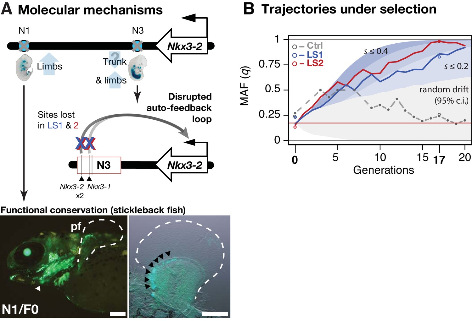
(A) At the Nkx3-2 locus, we identified two long-range enhancers, N1 and N3 (circles), located 600 and 230 kbp away, respectively. During development, they drive partially overlapping expression domains in limbs (N1 and N3) and trunk (N3), which are body regions that may correlate positively (tibia length) and possibly negatively (trunk with body mass) with the Longshanks selection regime. For both enhancers, the selected F17 alleles carry loss-of-function variants (gray crosses). Two out of three SNPs in the N3 F17 enhancer are predicted to disrupt an auto-feedback loop, likely reducing Nkx3-2 expression in the trunk and limb regions. Conversely, the enhancer function of the strong N1 F0 allele is evolutionarily conserved in fishes, demonstrated by its ability to drive consistent GFP expression (green) in the pectoral fins (pf, outlined) and branchial arches (white arrowhead, left) in transgenic stickleback embryos at 11 days post-fertilization. The N1 enhancer can recapitulate nkx3.2 expression in distal cells specifically in the endochondral radial domain in developing fins (black arrowheads, right). Scale bar: 250 µm for both magnifications. (B) Allele frequency of the selected allele (minor allele at F0, q) at N3 over 20 generations (blue: LS1; red: LS2; gray broken line: Ctrl; results from N1 were nearly identical due to tight linkage). Observed frequencies from genotyped generations in the Ctrl line are marked with filled circles. Dashed lines indicate missing Ctrl generations. Open circles at generations 0 and 17 indicate allele frequencies from whole genome sequencing. The allele frequency fluctuated in Ctrl due to random drift but followed a generally linear increase in the selected lines from around 0.17 to 0.85 (LS1) and 0.98 (LS2) by generation 17. Shaded contours mark expected allelic trajectories under varying selection coefficients starting from 0.17 (red horizontal line; the average starting allele frequency between LS1 and LS2 founders). The gray shaded region marks the 95% confidence interval under random drift.
Figure 5—figure supplement 1
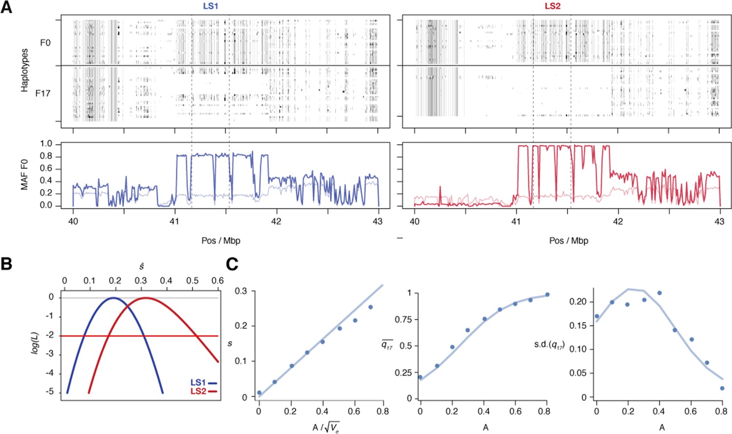
Selection at the Nkx3-2 locus.
(A) Raw genotypes from the F0 and F17 generations from LS1 (left) and LS2 (right) are shown, clearly indicating the area under the selective sweep. The genotype classes are shown as C57BL/6J homozygous (BL6, white), heterozygous (black) and alternate homozygous (dark gray). Lower Panel: Tracking MAF from both lines show that the originally rare F0 allele (thin line) rose to high frequency at F17 (thick lines). The plateau profile from both lines suggested that the same originally rare allele was segregating at in both founder populations and became very common by F17 in both lines (see raw genotypes). Note that in LS2 F17 the region is nearly fixed for the BL6 allele except in the bottom-most individual. (B) The log likelihood of the selection coefficient, s, for LS1 and LS2 (blue and red, respectively), based on transition probabilities for a Wright–Fisher population with the appropriate Ne. The horizontal red line shows a loss of log likelihood of 2 units, which sets conventional 2-unit support limits. (C) Simulations of an additive allele with effect A on the trait; 40 replicates for each value of A. Left: The selection coefficient, estimated from the change in mean allele frequency, as a function of ; the line shows the least-squares fit . Middle: dots show the mean allele frequency at generation 17; the line shows the prediction from the single-locus Wright–Fisher model, given . Right: the same, but for the standard deviation of allele frequency.
Tables
Table 1
Major loci likely contributing to the selection response.
These eight loci show significant allele frequency shifts in ∆z2 and are ordered according to their estimated selection coefficients according to Haldane (1932). Shown for each locus are the full hitchhiking spans, peak location and their size covering the core windows, the overlapping TAD and the number of genes found in it. The two top-ranked loci show shifts in parallel in both LS1 and LS2, with the remaining six showing line-specific response (LS1: 1; LS2: 5). Candidate genes found within the TAD with limb, cartilage, or bone developmental knockout phenotype functions are shown, with asterisks (*) marking those with a ‘short tibia’ knockout phenotype (see also Figure 2—figure supplement 3 and Supplementary file 3 for full table).
| Rk | Chr | Span (Mbp) | Peak | Core (kbp) | TAD (kbp) | Genes | ∆q | ||||
|---|---|---|---|---|---|---|---|---|---|---|---|
| LS1 | LS2 | Ctrl | Type | Candidate genes | |||||||
| 1 | 5 | 38.95–45.13 | 41.77 | 900 | 720 | 3 | 0.69 | 0.86 | −0.14 | Parallel | Nkx3-2 |
| 2 | 10 | 77.47–87.69 | 81.07 | 5360 | 6520 | 175 | 0.79 | 0.88 | −0.04 | Parallel | Sbno5, Aes, Adamtsl5*, Chst11*, Cry1, Prdm4* |
| 3 | 18 | 53.63–63.50 | 58.18 | 220 | 520 | 4 | 0.05 | 0.78 | −0.06 | LS2-specific | - |
| 4 | 13 | 35.59–55.21 | 48.65 | 70 | 2600 | 22 | 0.24 | 0.80 | −0.03 | LS2-specific | Id4 |
| 5 | 1 | 53.16–57.13 | 55.27 | 10 | 720 | 4 | 0.65 | 0.01 | −0.23 | LS1-specific | - |
| 6 | 15 | 31.92–44.43 | 41.54 | 10 | 680 | 3 | −0.23 | 0.66 | 0.02 | LS2-specific | Rspo2* |
| 7 | 6 | 118.65–125.25 | 120.30 | 130 | 1360 | 12 | −0.03 | 0.79 | −0.15 | LS2-specific | Wnt5b* |
| 8 | 11 | 111.10–115.06 | 113.42 | 10 | 2120 | 2 | −0.14 | 0.66 | −0.15 | LS2-specific | Sox9* |
-
Rk, Rank.
Chr, Chromosome.
-
Core, Span of 10 kbp windows above HINF, max LD p≤0.05 significance threshold.
TAD, Merged span of topologically associating domains (TAD) overlapping the core span. TADs mark segments along a chromosome that share a common regulatory mechanism. Data from Dixon et al. (2012).
-
Candidate genes, Genes within the TAD span showing ‘short tibia’, ‘short limbs’, ‘abnormal osteoblast morphology’ or ‘abnormal cartilage morphology’ knockout phenotypes are listed, with * marking those with ‘short tibia’.
Additional files
-
Supplementary file 1
Sequencing Summary.
For each line and generation, we individually barcoded all available individuals and pooled for sequencing. We aimed for a sequencing depth of around 100x coverage for 50–64 haplotypes per sample. Since the CD-1 mice were founded by an original import of 7 inbred females and two inbred males, we expect a maximum of 18 segregating haplotypes at any given locus. This sequencing design should give sufficient coverage to recover allele frequencies and possibly genotypes genome-wide. Our successful genome-wide imputation results validated this strategy.
- https://doi.org/10.7554/eLife.42014.019
-
Supplementary file 2
Pairwise FST and segregating sites (S) between populations.
As expected, there is a general trend of decrease in diversity after 17 generations of breeding. Globally, there was a 13% decrease in diversity, but F17 populations still retained on average ~5.8M segregating SNPs (diagonal). There was very little population differentiation, as indicated by low FST among the three founder populations, however FST increases by at least 100-fold among lines by generation F17 (above diagonal, orange boxes). Within-line FST is intermediate in this respect, reaching about half of the differentiation observed between lines.
- https://doi.org/10.7554/eLife.42014.020
-
Supplementary file 3
Full details on the eight discrete loci.
Listed here are the eight loci shown in Table 1, with additional details on the core span and the TAD span used to identify candidate genes, and a full list of genes within the full span.
- https://doi.org/10.7554/eLife.42014.021
-
Supplementary file 4
Detected protein-coding changes with large allele frequency shift in amino acids.
Listed are genes carrying large frequency changing SNPs affecting amino acid residues. Highlighted cells indicate the line with greater frequency changes ≥ 0.34 (red text with shading). Other suggestive changes are also shown with red numbers in unshaded cells. The changed amino acids are marked using standard notations, with the directionality indicated as ‘purifying’ or ‘diversifying’ with respect to a 60-way protein sequence alignment with other placental mammals. The conservation score based on phastCons was calculated at the SNP position itself, ranging from 0 (no conservation) to 1 (complete conservation) among the 60 placental mammals. For each gene, reported knockout phenotypes of the ‘limbs/digits/tail’ category is reported, along with whether lethality was reported in any of the alleles, excluding compound genotypes. A summary of the mutant phenotype as reported by the Mouse Genome Informatics database is also included to highlight any systemic defects beyond the ‘limbs/digits/tail’ category (lethal phenotypes reported in bold).
- https://doi.org/10.7554/eLife.42014.022
-
Supplementary file 5
Oligonucleotides for in situ hybridization probes.
- https://doi.org/10.7554/eLife.42014.023
-
Supplementary file 6
Oligonucleotide primers for multiplexed 4C-seq of enhancer viewpoints at the Nkx3-2 locus.
The 4C-seq adapter and adapter-specific primer sequences are given in Sexton et al. (2012). N2-DS denotes its location as 18 kbp downstream of the actual N2 enhancer. All viewpoints are pointed towards Nkx3-2 gene body ('+' strand).
- https://doi.org/10.7554/eLife.42014.024
-
Supplementary file 7
Oligonucleotide primers for amplifying the enhancers at the Nkx3-2 locus.
Each of the amplicons are tagged with SalI (forward) or XhoI (reverse) sites (underlined) for concatenation and flanked by EcoRV sites (underlined and bold) for insertion into the pBeta-lacZ-attBx2 reporter vector upstream of the β-globin minimal promoter.
- https://doi.org/10.7554/eLife.42014.025
-
Supplementary file 8
Oligonucleotide primers for allele-specific genotyping of the N3 enhancer.
The primers were designed to target two SNPs (bold) in the N3 enhancer, rs33219710 and rs33600994.
- https://doi.org/10.7554/eLife.42014.026
-
Transparent reporting form
- https://doi.org/10.7554/eLife.42014.027
Download links
A two-part list of links to download the article, or parts of the article, in various formats.
Downloads (link to download the article as PDF)
Open citations (links to open the citations from this article in various online reference manager services)
Cite this article (links to download the citations from this article in formats compatible with various reference manager tools)
An integrative genomic analysis of the Longshanks selection experiment for longer limbs in mice
eLife 8:e42014.
https://doi.org/10.7554/eLife.42014


