KymoButler, a deep learning software for automated kymograph analysis
- University of Cambridge, United Kingdom
Figures
Figure 1 with 5 supplements
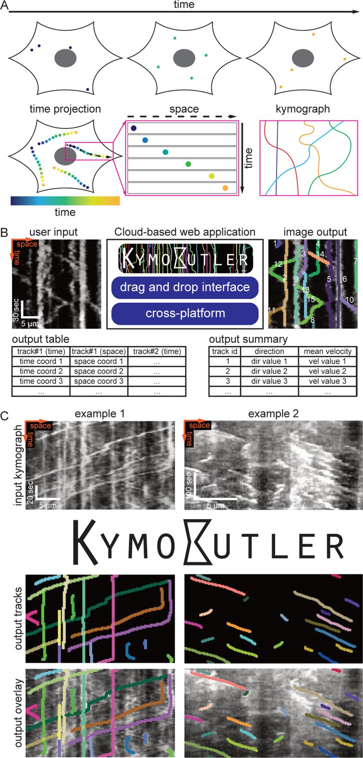
Kymograph generation and KymoButler.
Figure 1—figure supplement 1
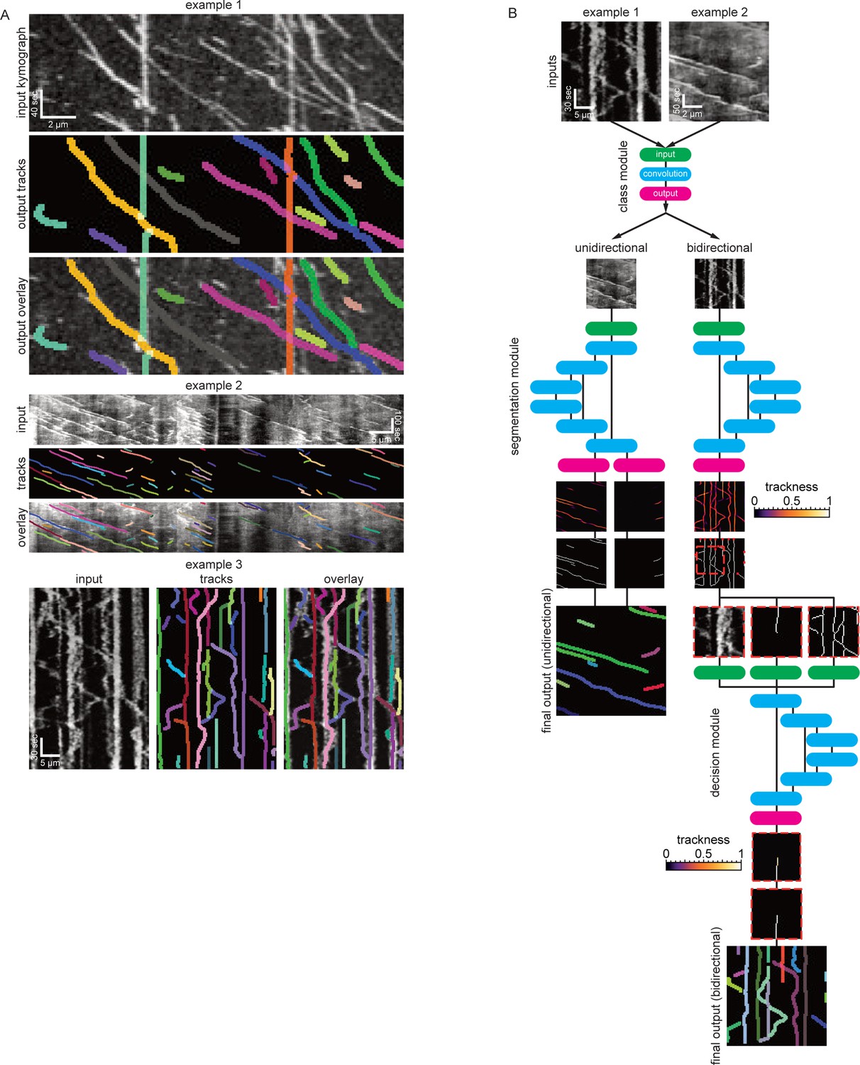
Example kymographs and software workflow.
(A) Three example kymographs from published manuscripts. Example 1: In vitro dynamics of single cytoplasmic dynein proteins adapted from Tanenbaum et al. (2013). Example 2: EB1-GFP labelled growing microtubule plus-ends in mouse dorsal root ganglion axons (Lazarus et al., 2013). Example 3: Mitochondria dynamics in mouse retinal ganglion cell dendrites (Faits et al., 2016). Each dilated coloured line depicts an identified track. (B) KymoButler software workflow. First, a classification module is applied to each kymograph to determine whether the kymograph is unidirectional or bidirectional. If the kymograph is deemed unidirectional the unidirectional segmentation module is applied to the image to generate two trackness maps that assign each pixel a score between 0–1, approximating the likelihood that this pixel is part of a track with negative slope (left image) or positive slope (right image). Subsequently, the trackness maps are binarized, skeletonised, and segmented into their respective connected components. Finally, those components are averaged over each row to generate individual tracks, and a dilated representation of each track is plotted in a random colour. If the kymograph is classified as bidirectional, another segmentation module is applied to the kymograph, which generates a trackness map that does not highlight any particular slope. This map is binarized with a user-defined threshold and subsequently skeletonised, resulting in a binary map that exhibits multiple track crossings. To resolve these crossings, we first apply a morphological operation that detects the starting points of tracks in the binary map (red dots). Then, the algorithm tracks each line from its starting point until a crossing is encountered. At each crossing, the decision module is called, whose inputs are (i) the raw kymograph in that region, (ii) the previous track skeleton, and (iii) all possible tracks in that region. The decision module then generates another trackness map that assigns high values to the most likely future path from the crossing. This map is then again binarized and thinned with a fixed threshold of 0.5. If the predicted path is longer than two pixels, the path tracking continues. Once all starting points have been tracked until an end (either no prediction or no further pixels available), the algorithm again looks for starting points in the skeletonised trackness map excluding the identified tracks, and repeats the steps outlined above until all pixels are occupied by a track. The resulting tracks are then drawn with each track in a random colour.
Figure 1—figure supplement 2
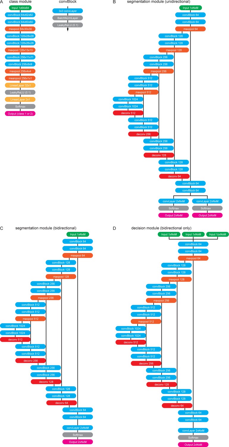
The software modules in detail.
(A) The class module. This module resizes any input kymograph to 64 × 64 pixels. It subsequently applies two convBlocks with no padding and 64 output feature maps to the image. ConvBlocks comprise a convolutional layer with 3 × 3 kernels followed by a BatchNormalisation Layer and a leaky Rectified Linear Unit (ReLU) activation function (leak factor 0.1). The convBlocks are followed by 2 × 2 max pooling to halve the feature map sizes. This is repeated another two times while steadily increasing the number of feature maps until the last convBlock generates 256 feature maps of size 9 × 9. These maps are then pooled with a final 2 × 2 max pool operation followed by a 4 × 4 mean pool operation to generate a vector of 256 features. These features are then classified with a fully connected layer with output nodes followed by another leaky Ramp and finally another fully connected layer generates two output values that correspond to the probability of being a unidirectional/bidirectional kymograph. (B) The unidirectional segmentation module takes and an input kymograph of arbitrary size. Subsequently two convBlocks with 64 output feature maps are applied to the image followed by max pooling. This is repeated three times while doubling the number of feature maps with each pooling operation forming the ‘contracting path’. To obtain an image of the same size as the input image the small feature maps at the lowest level of the network have to be deconvolved four times each time halving the number of feature maps and applying further convBlocks. After each 2 × 2 deconvolution the resulting feature maps are catenated with the feature maps of the same size from the contracting path so that the network only learns residual alterations of the input image. The final 64 feature maps are linked to two independent convolutional layers that generate outputs that correspond to the trackness scores for positive and negative sloped lines. (C) The bidirectional segmentation module has the same architecture as the unidirectional one but only generates one output that corresponds to the trackness map for any lines in the image. (D) The decision module architecture is the same as the bidirectional segmentation module but takes three input images instead of one.
Figure 1—figure supplement 3
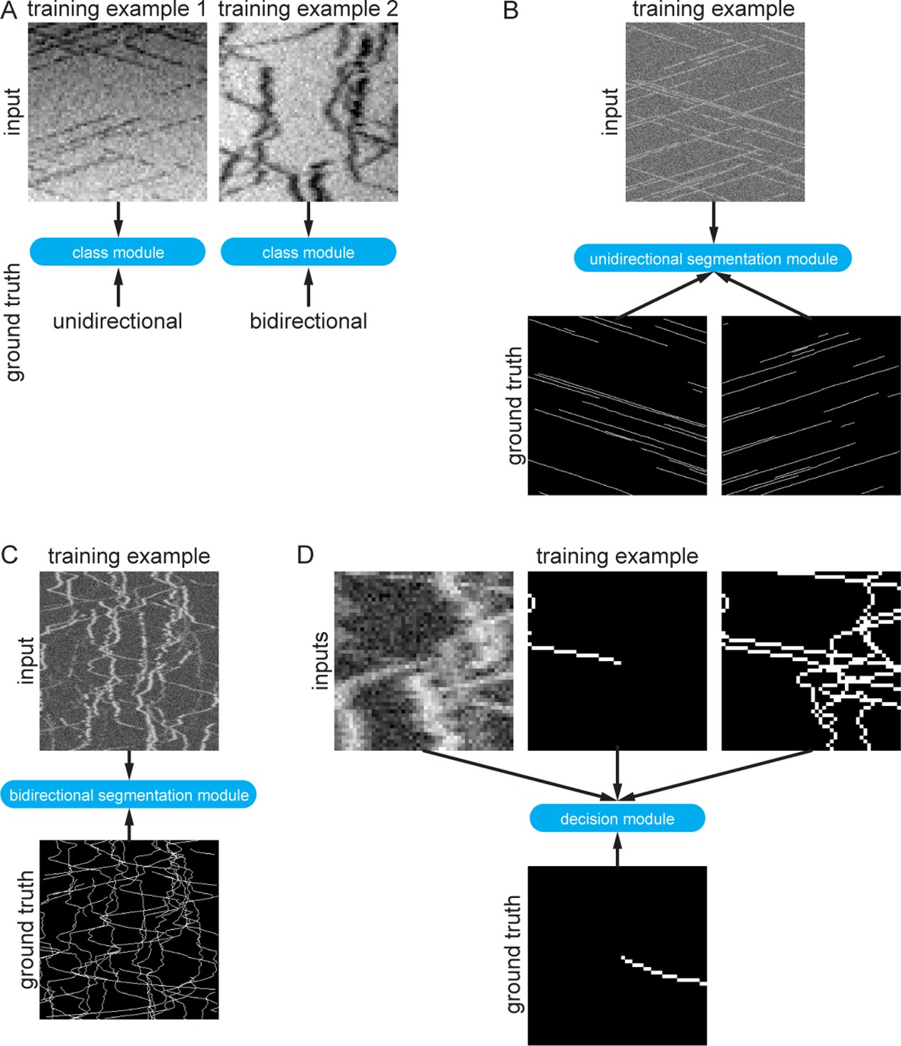
Synthetic training data examples.
(A) Class module training data consisted of 64 × 64 pixel images that were either classified as unidirectional (example 1) or bidirectional (example 2). (B) Synthetic training data for the unidirectional segmentation module comprised 300 × 300 pixel kymographs with two binary ground truth maps, corresponding to particle motion with negative and positive slopes. (C) Synthetic bidirectional segmentation module training data comprises 300 × 300 pixel kymographs with only one ground truth image containing all ground truth tracks. (D) The decision module was trained with 48 × 48 pixel image crops of the raw kymograph, the previous skeletonised path, and all the skeletonised paths in the cropped region. The ground truth is simply the known future segment of the given path.
Figure 1—figure supplement 4
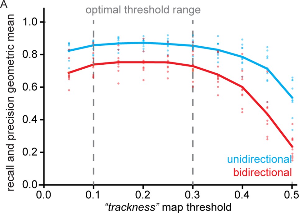
Geometric mean of track recall and precision for different trackness thresholds.
(A) 10 synthetic unidirectional and bidirectional kymographs were analysed with varying trackness thresholds, and track recall and track precision were calculated. The geometric mean of recall and precision does not exhibit much variation between 0.1 and 0.3 but decreases at lower and higher values. Individual dots represent per kymograph values and the solid lines the binned mean.
Figure 1—figure supplement 5
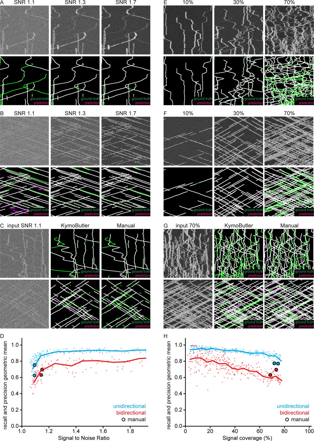
Geometric mean of track recall and precision for different signal to noise ratios and particle densities.
(A, B) The same synthetic (A) bidirectional and (B) unidirectional kymograph for three different SNR values (top). Note that some tracks become almost invisible at low SNRs. Bottom: Overlay of the tracks predicted by KymoButler (magenta, not post processed) with the ground truth (green). (C) A low SNR unidirectional/bidirectional kymograph analysed by KymoButler and manual annotation. Predicted tracks in magenta and ground truth in green. (D) The geometric mean of track recall and precision as a function of SNR. The same 10 kymographs were noised with different SNRs and the average score taken. Dots represent individual kymographs and the line the 0.1 bin average. Highlighted dots represent manually analysed kymographs. (E, F) Three example (E) bidirectional and (F) unidirectional kymographs for different particle densities (top). The percentage value gives the percentage of the image covered with signal. Bottom: Overlay of the tracks predicted by KymoButler (magenta) with the ground truth (green). (G) A high particle density unidirectional/bidirectional kymograph analysed with KymoButler and manual annotation. Predicted tracks in magenta and ground truth in green. (H) The geometric mean of track recall and precision as a function of coverage percentage. 20 kymographs were generated with varying numbers of particles. Tracks smaller than three pixels and shorter than three frames were discarded for unidirectional kymograph quantification while tracks smaller than 10 pixels and shorter than 25 frames were discarded for bidirectional kymograph quantification. Dots represent individual kymographs and the line the 5% bin average. Highlighted dots represent manually analysed kymographs.
Figure 2 with 1 supplement
Benchmark of KymoButler against unidirectional synthetic data.
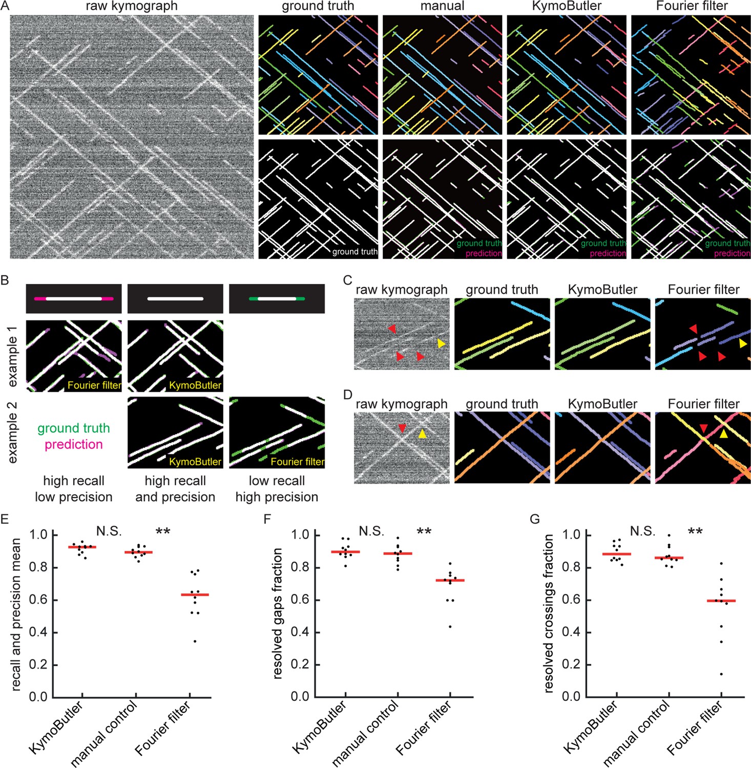
(A) An example synthetic kymograph and its corresponding ground truth, manual control, the prediction by KymoButler, and the prediction by Fourier filtering. The top row depicts individual tracks in different colours and the bottom row shows the prediction overlay (magenta) with the ground truth (green) for all approaches. Discrepancies are thus highlighted in magenta (false positive) and green (false negative), while matching ground truth and prediction appears white. (B) Schematic explaining the concept of recall and precision. The top row depicts the possible deviations of the prediction from the ground truth. The middle and bottom rows show example overlays, again in green and magenta, from the synthetic data. In the left column, the prediction is larger than the ground truth (magenta is visible) leading to false positive pixels and low track precision, but a small number of false negatives and thus high track recall. An example prediction overlay of the Fourier filter approach is shown, which tends to elongate track ends. The right column shows a shorter prediction than the ground truth, leading to green segments in the overlay. While this prediction has high track precision (low number of false positive pixels), track recall is low due to the large number of false negatives. Again, a cut-out from the Fourier filter prediction is shown, where multiple gaps are introduced in tracks, thus severely diminishing track recall (see Material and methods for a detailed explanation of recall and precision). The middle column shows the same two cut outs analysed by KymoButler. No magenta or green segments are visible, thus leading to high recall and precision. (C) Synthetic kymograph region with four gaps highlighted (arrow heads): in one or more kymograph image rows the signal was artificially eliminated but kept in the ground truth to simulate real fluorescence data. While KymoButler efficiently connects tracks over gaps, the Fourier filter is unable to do so and breaks up those tracks into segments or incorrectly shortens these tracks (red arrow heads). Yellow arrow heads depict correct gap bridging events. (D) A synthetic kymograph with several line crossings. While KymoButler efficiently resolved all crossings, that is lines that cross other lines are not broken up into two segments, the Fourier filter correctly identifies the line crossing at the yellow arrow head but erroneously terminates the red and yellow tracks at the red arrow head. (E) The geometric means of recall and precision (‘track F1 score’) for KymoButler, the Fourier filter approach, and manual control. Each dot represents the average track F1 score of one synthetic kymograph (, Kruskal-Wallis Test, Tukey post-hoc: manual vs KymoButler , manual vs Fourier Filtering ). (F) Quantification of gap bridging performance for KymoButler (89%), manual control (88%), and Fourier filter (72%); lines: medians of all 10 synthetic kymographs, , Kruskal-Wallis Test, Tukey post-hoc: manual vs KymoButler , manual vs Fourier Filtering . (G) The fraction of correctly identified crossings for KymoButler, manual annotation, and the Fourier filter (88% KymoButler, 86% manual, 60% Fourier filter; lines: medians of all 10 synthetic kymographs, , Kruskal-Wallis Test, Tukey post-hoc: manual vs KymoButler , manual vs Fourier Filtering ). Tracks smaller than 3 pixels and shorter than 3 frames were discarded from the quantification.
-
Figure 2—source data 1
Table of presented data.
A CSV file that contains: the average track F1 score, the average gap score, and the average crossing score for each unidirectional synthetic kymograph.
- https://cdn.elifesciences.org/articles/42288/elife-42288-fig2-data1-v2.csv
-
Figure 2—source data 2
Synthetic kymographs and movies.
A ZIP file containing all analysed synthetic unidirectional movies, their kymographs, results from KymographClear based analysis and manually annotated ImageJ rois.
- https://cdn.elifesciences.org/articles/42288/elife-42288-fig2-data2-v2.zip
Figure 2—figure supplement 1
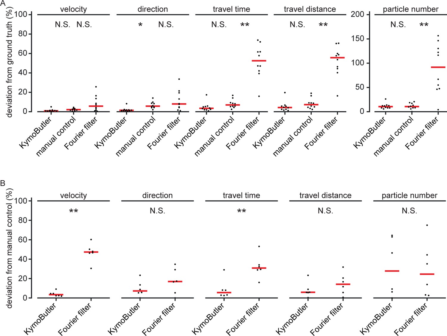
Data quantities derived from unidirectional kymographs using manual annotation, KymoButler, and Fourier filtering for simulated and real data.
(A) Deviation from the average ground truth values per synthetic kymograph for all three different analysis approaches (velocity: , Kruskal-Wallis Test, Tukey post-hoc: manual vs KymoButler , manual vs Fourier Filtering ; orientation: , manual vs KymoButler , manual vs Fourier Filtering ; travel time:, manual vs KymoButler , manual vs Fourier Filtering ; travel distance: , manual vs KymoButler , manual vs Fourier Filtering ; particle number: , manual vs KymoButler , manual vs Fourier Filtering ). (B) Deviation from manually obtained average values per real kymograph from our validation set (velocity: , Wilcoxon ranksum test; orientation: ; travel time: ; travel distance: ; particle number: ).
Figure 3 with 2 supplements
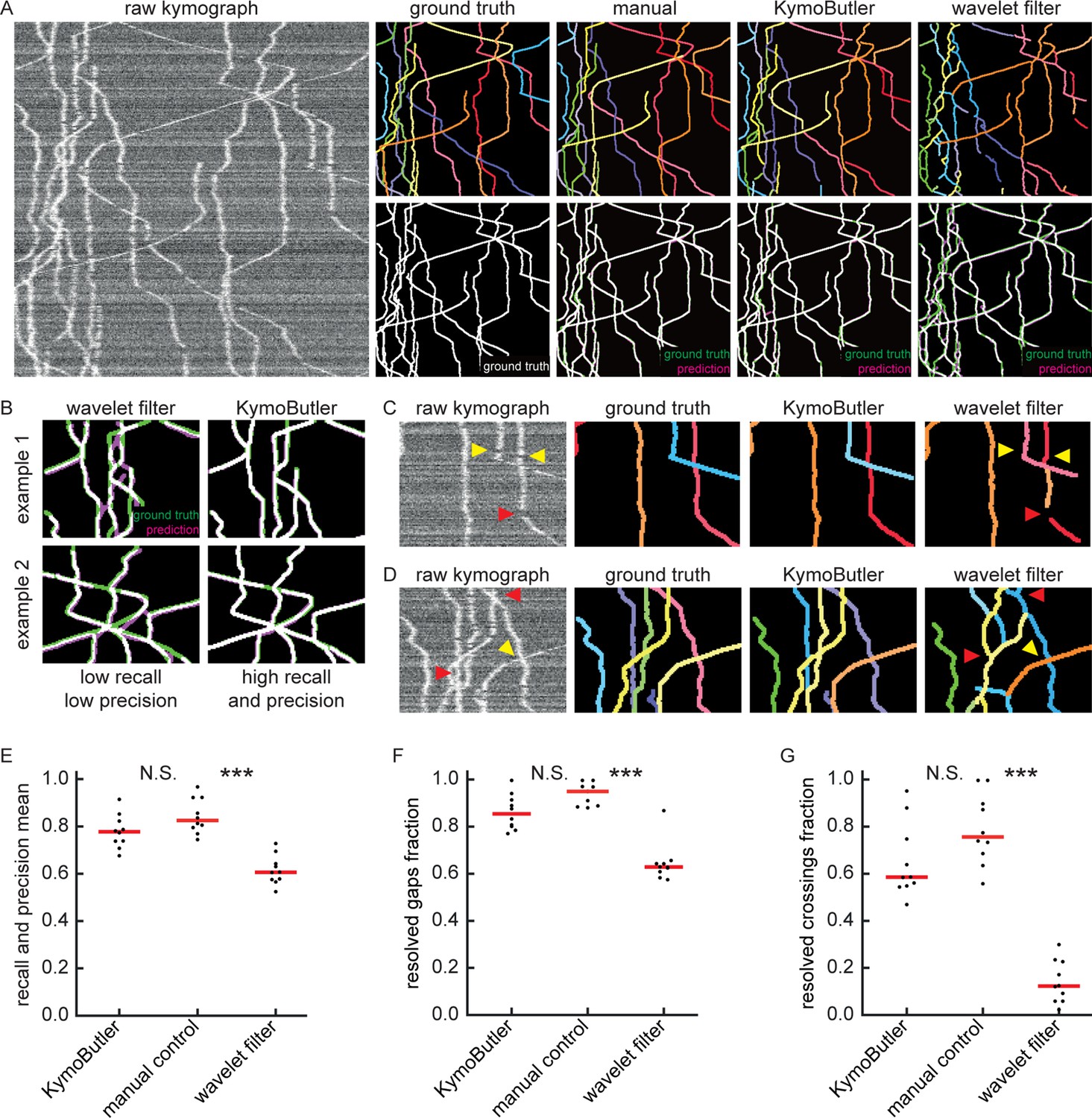
Benchmark of KymoButler against complex bidirectional synthetic data.
(A) Example synthetic kymograph and its corresponding ground truth, manual control, the prediction by KymoButler, and the prediction via wavelet coefficient filtering. The top row depicts individual tracks in different colours and the bottom row shows the prediction overlay (magenta) with the ground truth (green) for all approaches. Discrepancies are highlighted in magenta (false positive) and green (false negative), while the match of ground truth and prediction appears white. (B) Example recall and precision of KymoButler and wavelet filtering. While KymoButler shows high recall and high precision, the wavelet filter approach yields significant deviations from the ground truth (green and magenta pixels). (C) Synthetic kymograph region with three artificial gaps highlighted (arrow heads). While KymoButler efficiently connects tracks over gaps, the wavelet filter is unable to do so and breaks up those tracks into segments (red arrow heads). The yellow arrow heads depict correct gap bridging events. (D) A synthetic kymograph with several line crossings. While KymoButler efficiently resolved all crossings, that is lines that cross other lines are not broken up into segments, the wavelet filter only resolves one crossing correctly (yellow arrow head). (E) The geometric means of track recall and track precision (track F1 score) for KymoButler, manual control, and the wavelet filter. Each dot represents the average F1 score of one synthetic kymograph (, Kruskal-Wallis Test, Tukey post-hoc: manual vs KymoButler , manual vs wavelet filtering ). (F) Quantification of gap performance for KymoButler, manual annotation, and wavelet filter (, Kruskal-Wallis Test, Tukey post-hoc: manual vs KymoButler , manual vs wavelet filtering ). (G) The fraction of resolved crossings for KymoButler, manual control, and the wavelet filter (, Kruskal-Wallis Test, Tukey post-hoc: manual vs KymoButler , manual vs wavelet filtering ). KymoButler identifies tracks in complex kymographs as precisely as manual annotation by an expert.
-
Figure 3—source data 1
Table of presented data.
A CSV file that contains: the average track F1 score, the average gap score, and the average crossing score for each bidirectional synthetic kymograph.
- https://cdn.elifesciences.org/articles/42288/elife-42288-fig3-data1-v2.csv
-
Figure 3—source data 2
Synthetic kymographs and movies.
A ZIP file containing all analysed synthetic bidirectional movies, their kymographs, and manually annotated ImageJ rois.
- https://cdn.elifesciences.org/articles/42288/elife-42288-fig3-data2-v2.zip
Figure 3—figure supplement 1
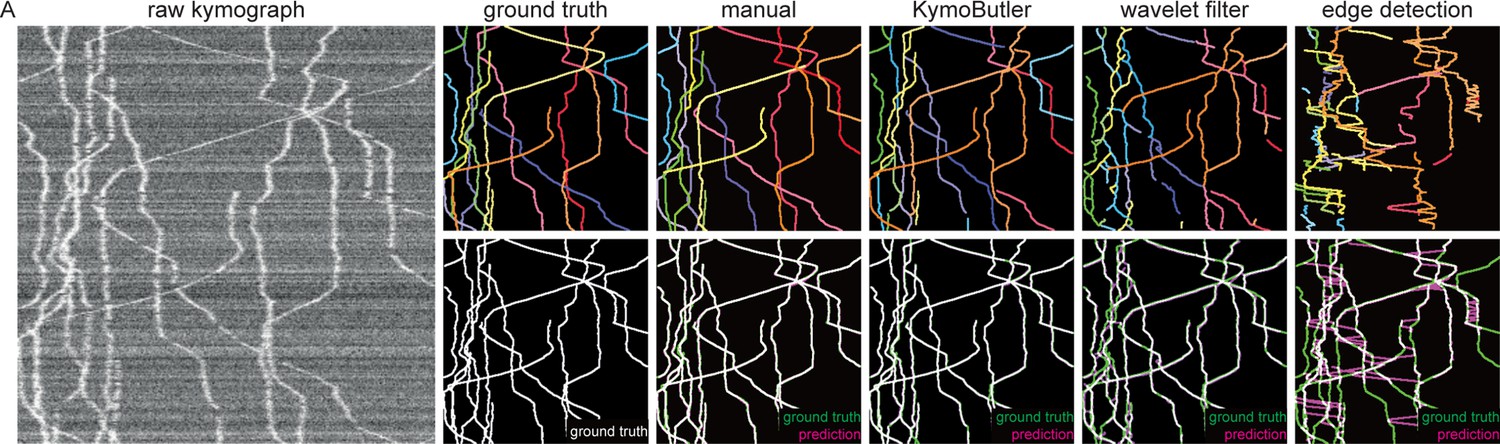
Performance of different skeletisation techniques on a synthetic bidirectional kymograph.
(A) Example of a synthetic bidirectional kymograph and its corresponding ground truth, the predictions by manual annotation, KymoButler, wavelet coefficient filtering, and tracks detected through edge filtering. The top row depicts individual tracks in different colours and the bottom row shows the prediction overlay (magenta) with the ground truth (green) for both approaches. Discrepancies are highlighted in magenta (false positive) and green (false negative), while a match of ground truth and prediction appears white.
Figure 3—figure supplement 2
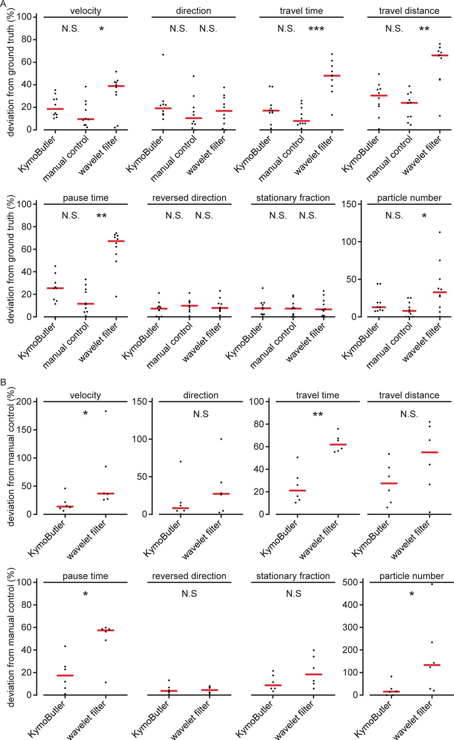
Synthetic data quantities derived from bidirectional kymographs using manual annotation, KymoButler, and wavelet filtering for simulated and real data.
(A) Deviation from the average ground truth values per synthetic kymograph for all three different analysis approaches (velocity: , Kruskal-Wallis Test, Tukey post-hoc: manual vs KymoButler , manual vs Wavelet Filtering ; orientation: ; travel time: , manual vs KymoButler , manual vs Wavelet Filtering ; travel distance: , manual vs KymoButler , manual Wavelet Filtering ; pause time: , manual vs KymoButler , manual Wavelet Filtering ; percentage of tracks that change direction at least once: ; percentage of stationary tracks: ; particle number: , manual vs KymoButler , manual vs Wavelet Filtering ). (B) Deviation from manually obtained average values per real kymograph from our validation set (velocity: , Wilcoxon ranksum test; orientation: ; travel time: ; travel distance: ; pause times: ; percentage of tracks that change direction at least once: ; percentage of stationary tracks per kymograph: ; particle number per kymograph: ).
Author response image 1
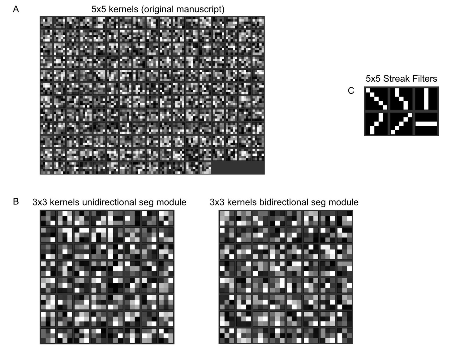
Normalised kernel entries of our fully convolutional neural network.
(A) Normalised 5x5 kernels from the first layer of the network from our original manuscript. (B) Normalised 3x3 kernels from the first layer of our unidirectional/bidirectional module. (C) Example 5x5 streak filters. The values run from 0 (black) to 1 (white). No obvious line filter structure is visible in our kernels.
Author response image 2
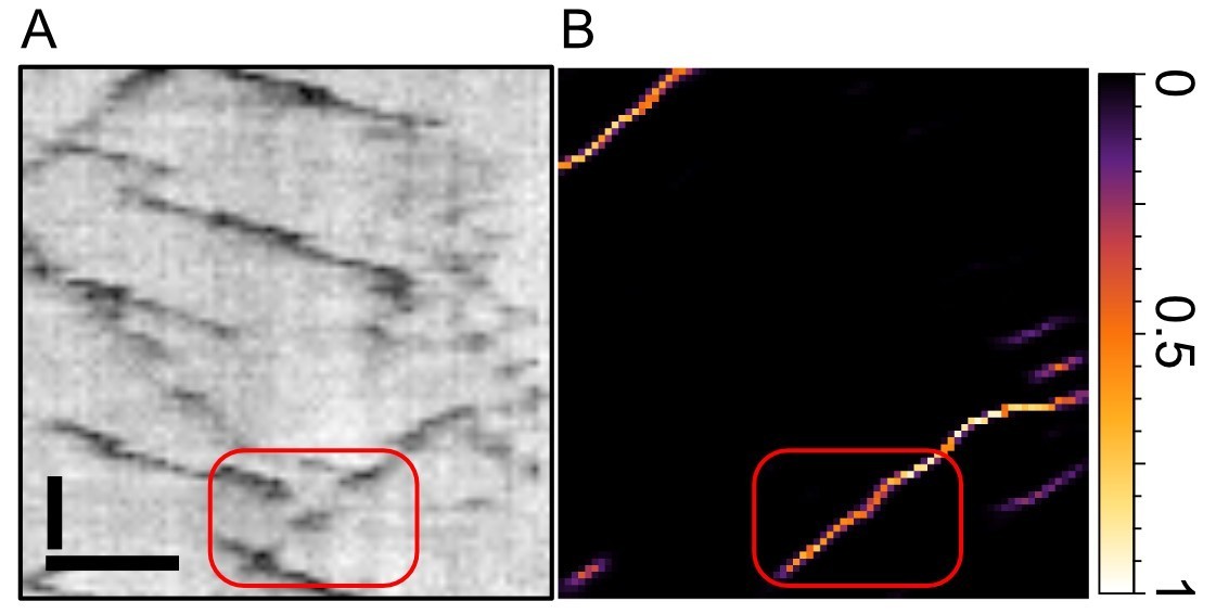
Zoom into the old Figure 1E from our manuscript.
(A) depicts the raw kymograph and (B) the pixel score map from our neural network. The track highlighted in red exhibits two gaps where the particle becomes invisible for three frames each. As seen in (B), the network has no problem to bridge those gaps and assign high scores throughout the gap. Scale bars 2 µm (horizontal), 25 sec vertical. See also our new Figures 2 and 3, where we benchmark KymoButler (and its capability to bridge gaps) against ground truth data.
Author response image 3
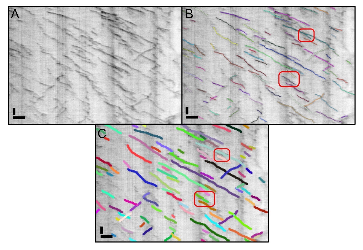
The kymograph shown in Figure 2 of our original manuscript analysed with the original KymoButler and the new version.
We highlighted the two errors we could identify in the old version in panel B (red frames). In the upper one, a junction was not resolved properly, and in the lower one two lines were so close to each other that they were segmented as one. Neither of these errors showed up when we re-ran the data in the new KymoButler. Scale bars: 2 µm (horizontal), 25 sec (vertical).
Author response image 4
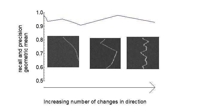
Track recall and precision as a function of number of particle direction changes.
Tables
Key resources table
| Resource | Designation. | Source. | Identifiers. | Additional information |
|---|---|---|---|---|
| Software, algorithm | MATLAB | MATLAB | RRID:SCR_001622 | Used for statistical analysis |
| Software, algorithm | Fiji | Fiji is Just ImageJ (https://fiji.sc) | RRID:SCR_002285 | Used to generate and analyse kymographs with KymographClear/Direct https://sites.google.com/site/kymographanalysis/ |
| Software, algorithm | Wolfram Mathematica | Wolfram Mathematica | RRID:SCR_014448 | Code available under https://github.com/MaxJakobs/KymoButler (copy archived at swh:1:rev:e35173e9051eb5395f9b13dcd8f487ffa4098592) |
Additional files
Download links
A two-part list of links to download the article, or parts of the article, in various formats.
Downloads (link to download the article as PDF)
Open citations (links to open the citations from this article in various online reference manager services)
Cite this article (links to download the citations from this article in formats compatible with various reference manager tools)
KymoButler, a deep learning software for automated kymograph analysis
eLife 8:e42288.
https://doi.org/10.7554/eLife.42288


