Protein denaturation at the air-water interface and how to prevent it
- Max Planck Institute of Biophysics, Germany
- Goethe University Frankfurt, Germany
- Sofja Kovalevskaja Group, Max Planck Institute of Biophysics, Germany
Figures
Figure 1 with 2 supplements
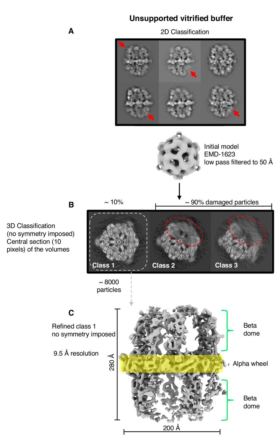
Single-particle cryo-EM results from unsupported vitrified buffer.
(A) Two-dimensional classification of particles shows weak or absent density of beta-domes (red arrows). (B) The alpha-wheel structure reveals major damage to about 90% of particles (dashed red). The remaining ∼10% (dashed grey) contributed to a reconstruction (C) at 9.5 Å resolution.
Figure 1—figure supplement 1
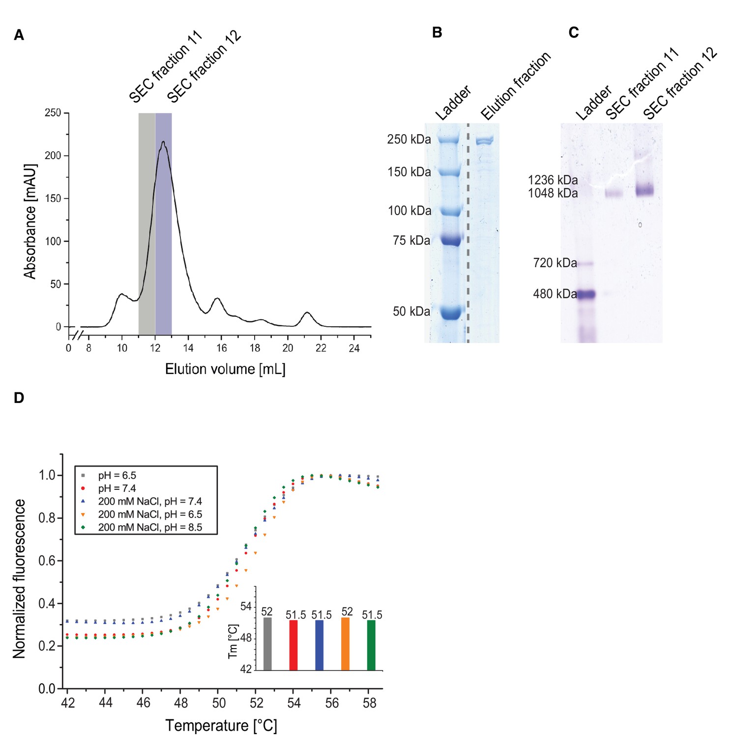
Purification and stability of yeast FAS.
(A) Size-exclusion chromatography. (B) SDS PAGE. (C) Blue-native PAGE. (D) Thermal shift assays in different buffers as a function of temperature. Columns show the average melting temperature of three replicates.
Figure 1—figure supplement 2
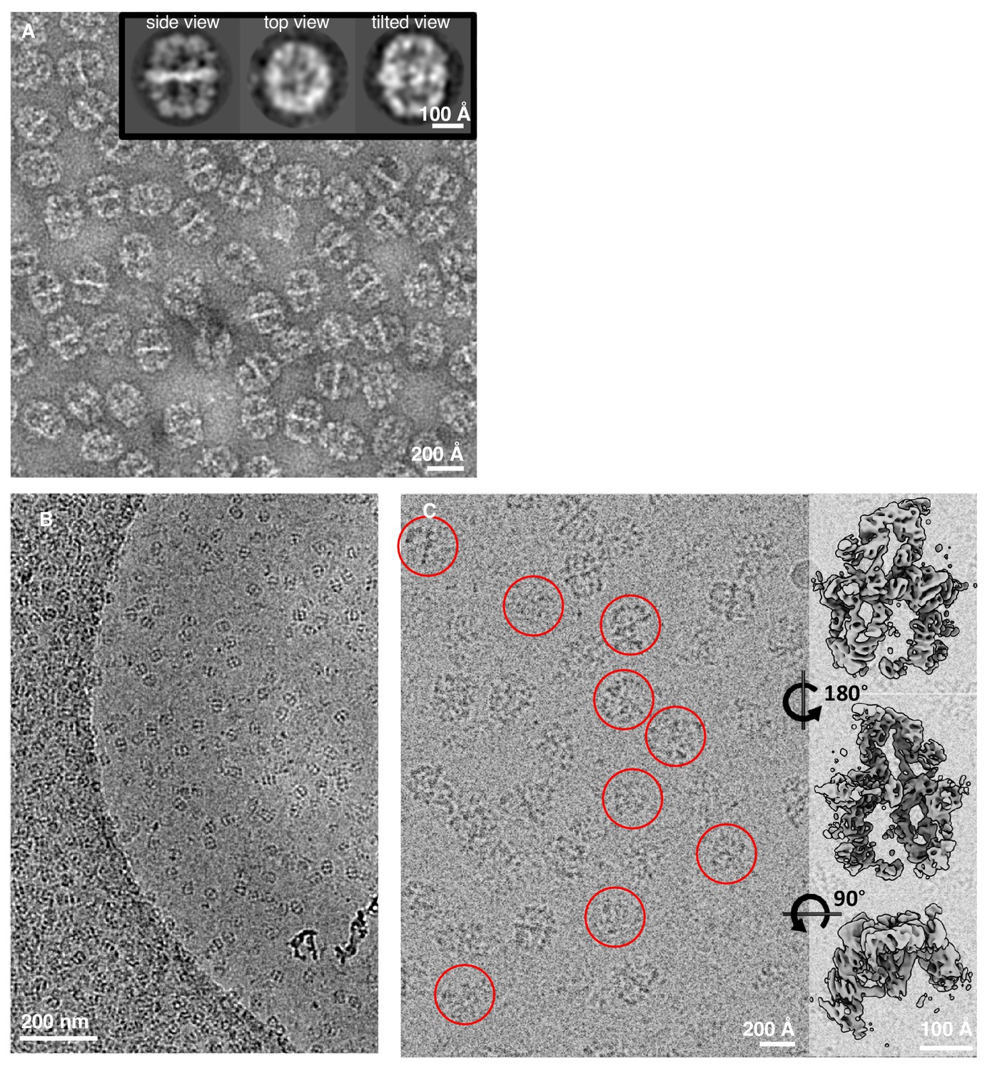
Comparison of FAS in negatively stained and unsupported cryo-EM specimens.
(A) Negatively stained FAS. The inset shows three representative 2D class averages. (B) Low magnification of a Quantifoil R2/2 cryo grid hole. (C) Broken particles from class 3 (Figure 1B) identified in a micrograph at higher magnification (red circles) and surface views of the corresponding three-dimensional reconstruction.
Figure 2 with 2 supplements
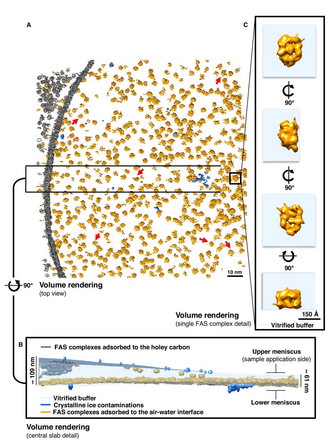
Particle distribution and structure of FAS in unsupported vitrified buffer.
(A) Segmentation of a typical Quantifoil R2/2 grid hole with FAS complexes. Red arrows indicate fragments of FAS particles. (B) Slab of vitrified buffer, delimited by carbon and small contaminating ice crystals. (C) Detail of a single FAS complex showing morphological differences between sides facing the air-water interface or away from it.
Figure 2—figure supplement 1
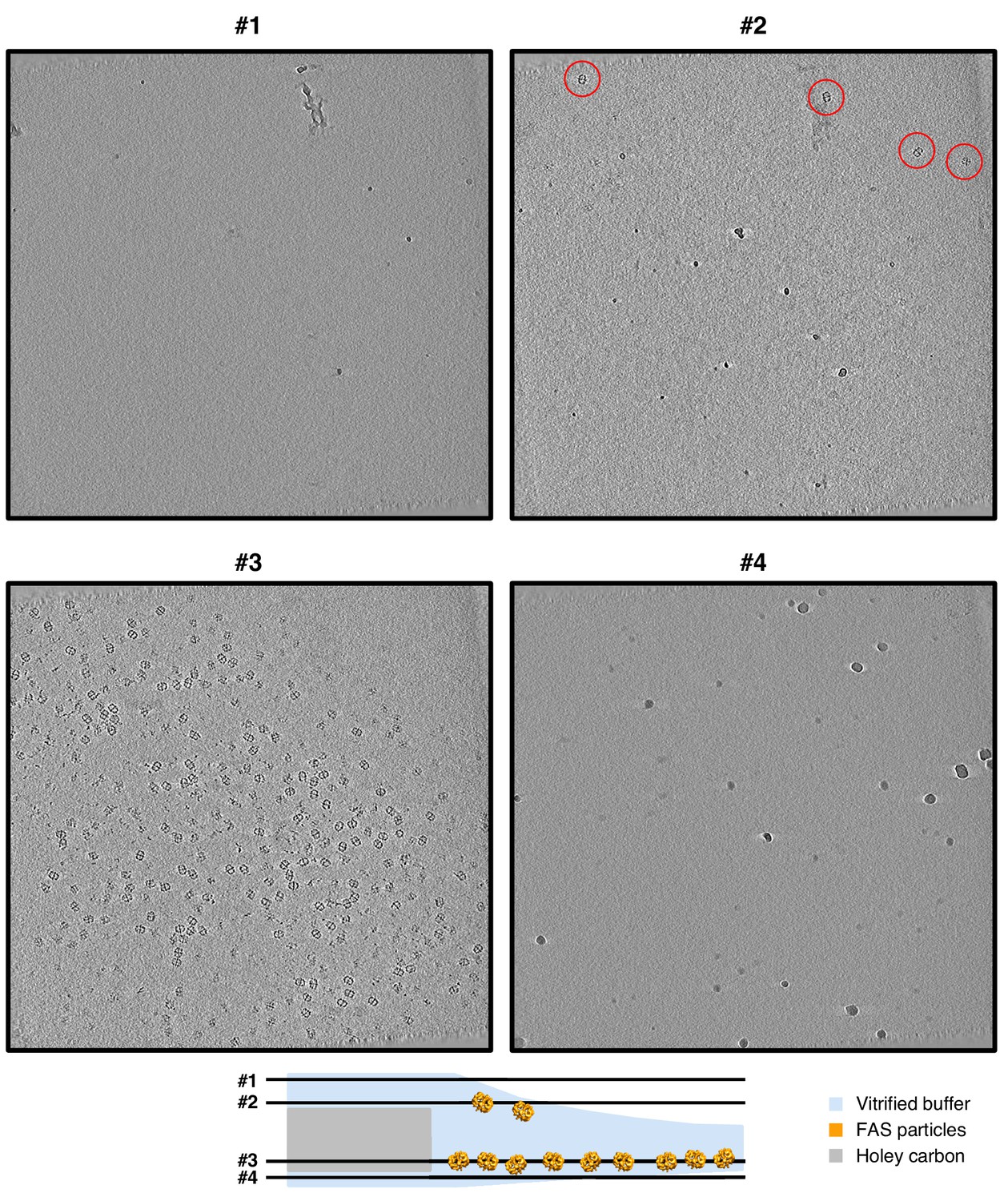
Slices through a tomogram of a Quantifoil hole with unsupported vitrified solution.
Four- pixel slices through NAD-filtered tomogram indicate atmospheric surface contamination by ice crystals (slices #1 and #4). The upper meniscus (slice #2) is less populated with adsorbed FAS particles (red circles) than the lower meniscus (slice #3).
Figure 2—video 1
Three-dimensional rendering of FAS in unsupported vitrified solution.
Tomographic reconstruction of the sample in Figure 2. The distribution of FAS particles is visible in the sequence of xy and xz slices and volume segmentation.
Figure 3 with 1 supplement
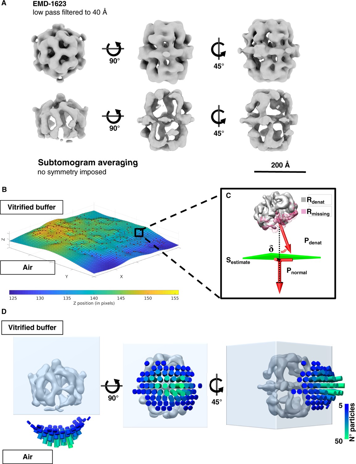
Sub-tomogram averaging and orientation of denatured FAS in unsupported vitrified buffer.
(A) Subtomogram averaging confirms localized denaturation of FAS. The published cryo-EM structure of intact FAS (Gipson et al., 2010) (above) is shown for comparison. (B) Surface (Sestimate) through the center of all FAS complexes in the selected area. (C) Vector Pdenat describing the orientation of denatured FAS (Rdenat), of the missing density (Rmissing) and the perpendicular direction (Pnormal) relative to Sestimate. The displacement angle is δ. (D) Angular distribution of δ for all particles in reconstructed tomograms.
Figure 3—figure supplement 1
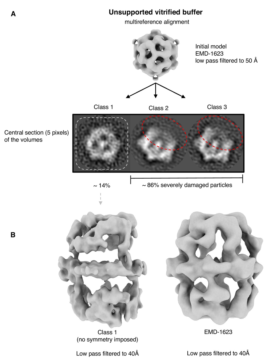
Multi-reference alignment of FAS in unsupported vitrified solution.
(A) Classification by MRA indicates FAS denaturation comparable to single-particle results (Figure 1B). Particles reconstructed from the best class (class 1) indicated significant denaturation (B). Published cryo-EM map of FAS (Gipson et al., 2010) shown for comparison on the right.
Figure 4
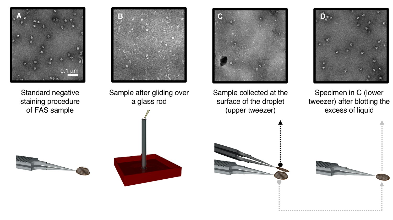
Denaturation by controlled exposure to air as analyzed by negative-stain EM.
(A) Untreated FAS sample (control). (B) A thin film of FAS solution flowing over a glass rod. Most complexes are denatured. (C) Denatured FAS particles picked up from the top of the droplet. (D) Undamaged FAS particles adsorbed to amorphous carbon at the opposite drop surface.
Figure 5 with 6 supplements

Sub-tomogram averaging of FAS vitrified on hydrophilized graphene.
(A) Zero degree view of tomographic tilt series. (B) Slab of vitrified buffer delimited by carbon and ice contaminants, indicating adsorption of FAS complexes to the graphene-water interface. (C) Subtomogram averaging confirms the structural integrity of FAS. (D) Three-dimensional impression (not drawn to scale) indicating the relative position of Quantifoil carbon film (dark grey) and hydrophilized graphene (mid-grey) on the copper support grid (dark red). The solution containing FAS particles (light grey) was applied from the uncoated side of the grid.
Figure 5—figure supplement 1
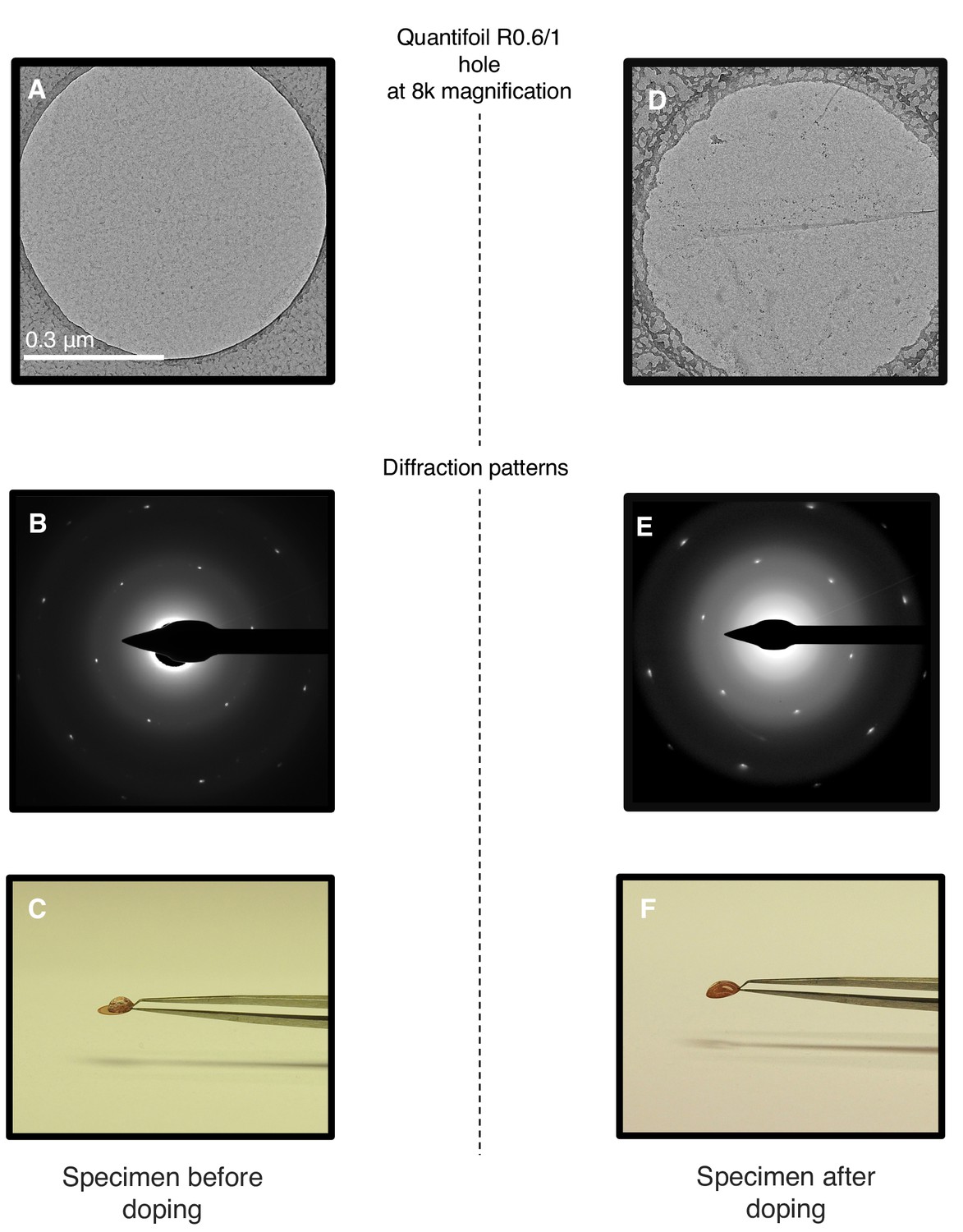
Chemical doping of graphene-coated Quantifoil grids.
(A) Quantifoil R0.6/1 grid coated with graphene. (B) Electron diffraction pattern of the area shown in (A). (C) Same grid with a droplet of water. (D) Same grid as in (A) after chemical doping with 1-pyrCA. (E) Electron diffraction pattern of area imaged in (D). (F) Doped grid with a droplet of water.
Figure 5—figure supplement 2
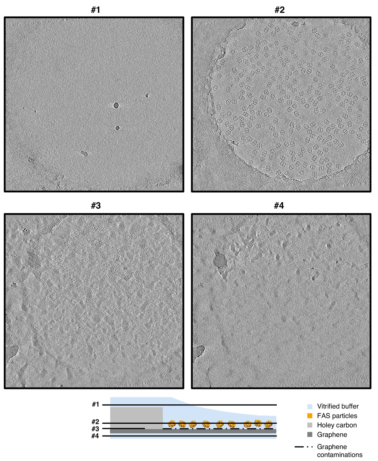
Slices through tomographic volume of FAS on hydrophilized graphene.
Four-pixel slices through NAD-filtered tomograms at various heights show atmospheric ice contamination (slices #1 and #4). FAS particles are evenly spread in one layer (slice #2) on the graphene film. A layer of contaminants on the lower surface identifies the position of the electron-transparent graphene sheet (slice #3).
Figure 5—figure supplement 3
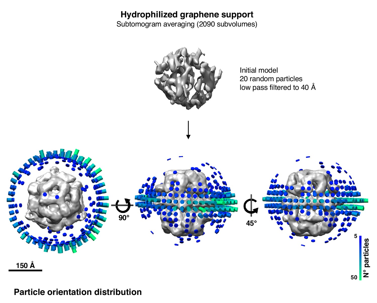
Angular distribution plot after subtomogram averaging of the particle dataset on hydrophilized graphene support (Figure 5C).
https://doi.org/10.7554/eLife.42747.014
Figure 5—figure supplement 4
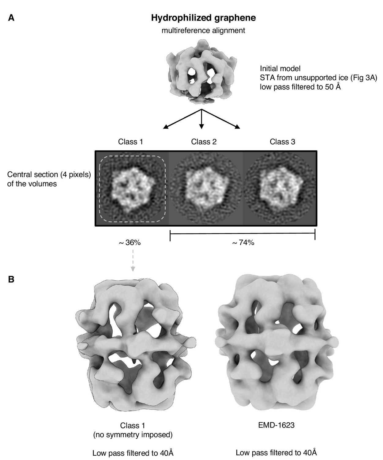
Multi-reference alignment of FAS on hydrophilized graphene.
Classification by MRA (A) indicates that all particles are intact. The map of the best class (class 1) does not show any sign of denaturation (B). Published cryo-EM map of FAS (Gipson et al., 2010) shown for comparison on the right.
Figure 5—figure supplement 5
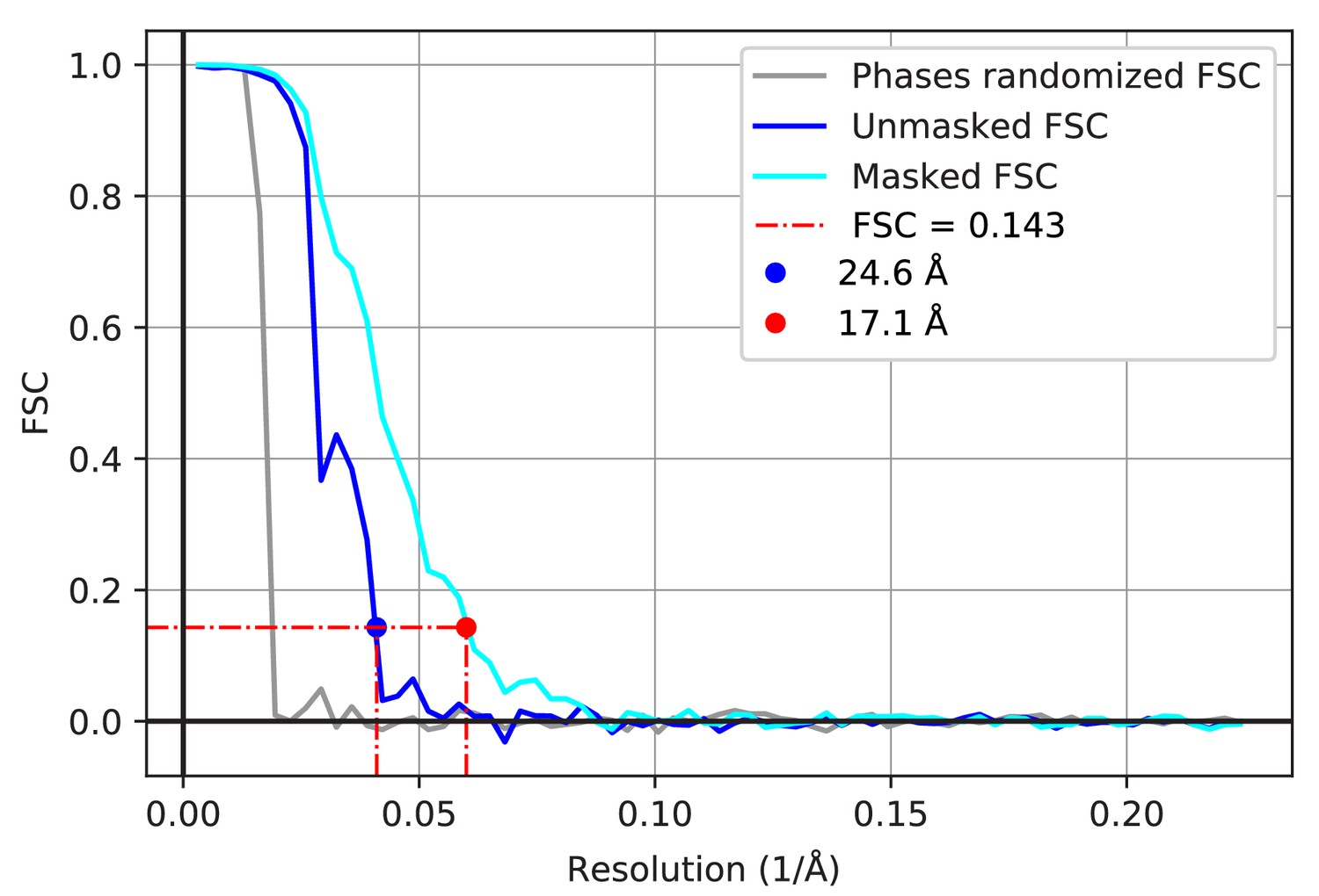
Resolution estimate of subtomogram averages.
FSC of the two unfiltered half-maps of FAS before (blue) and after (cyan) masking. FSC performed on the half-maps with phases randomized beyond 60 Å (grey). FSC curves before and after masking indicate resolutions of 24.6 Å and 17.1 Å, respectively.
Figure 5—video1
Three-dimensional rendering of FAS on hydrophilized graphene.
Tomographic reconstruction of sample in Figure 5. The distribution of FAS particles is visible in the sequence of xy and xz slices and volume segmentation. Holey carbon film (light gray), FAS (orange), graphene contamination (dark grey), atmospheric ice contamination (dark blue) and vitreous buffer (cyan). Density map and orientations from subtomogram averaging were used to place copies of FAS into the tomographic reconstruction. Vertical section: single layer of particles adsorbed to the graphene-water interface.
Figure 6 with 5 supplements

Single-particle cryo-EM results on hydrophilized graphene.
Two-dimensional (A) and three-dimensional (B) classification both show intact particles. A final map calculated without (C) or with (D) imposed D3 symmetry indicated a resolution of 4.8 Å or 4.0 Å.
Figure 6—figure supplement 1
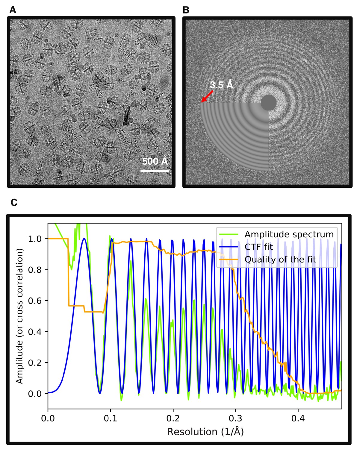
Hydrophilized graphene supported grids.
(A) Typical image of FAS vitrified on hydrophilized graphene. (B) Two-dimensional power spectrum of (A) extends beyond the highest frequency used to fit the theoretical CTF (3.5 Å). (C) Rotationally averaged one-dimensional plot of (B) shows that the CTF fit extends beyond 3 Å spatial frequency.
Figure 6—figure supplement 2
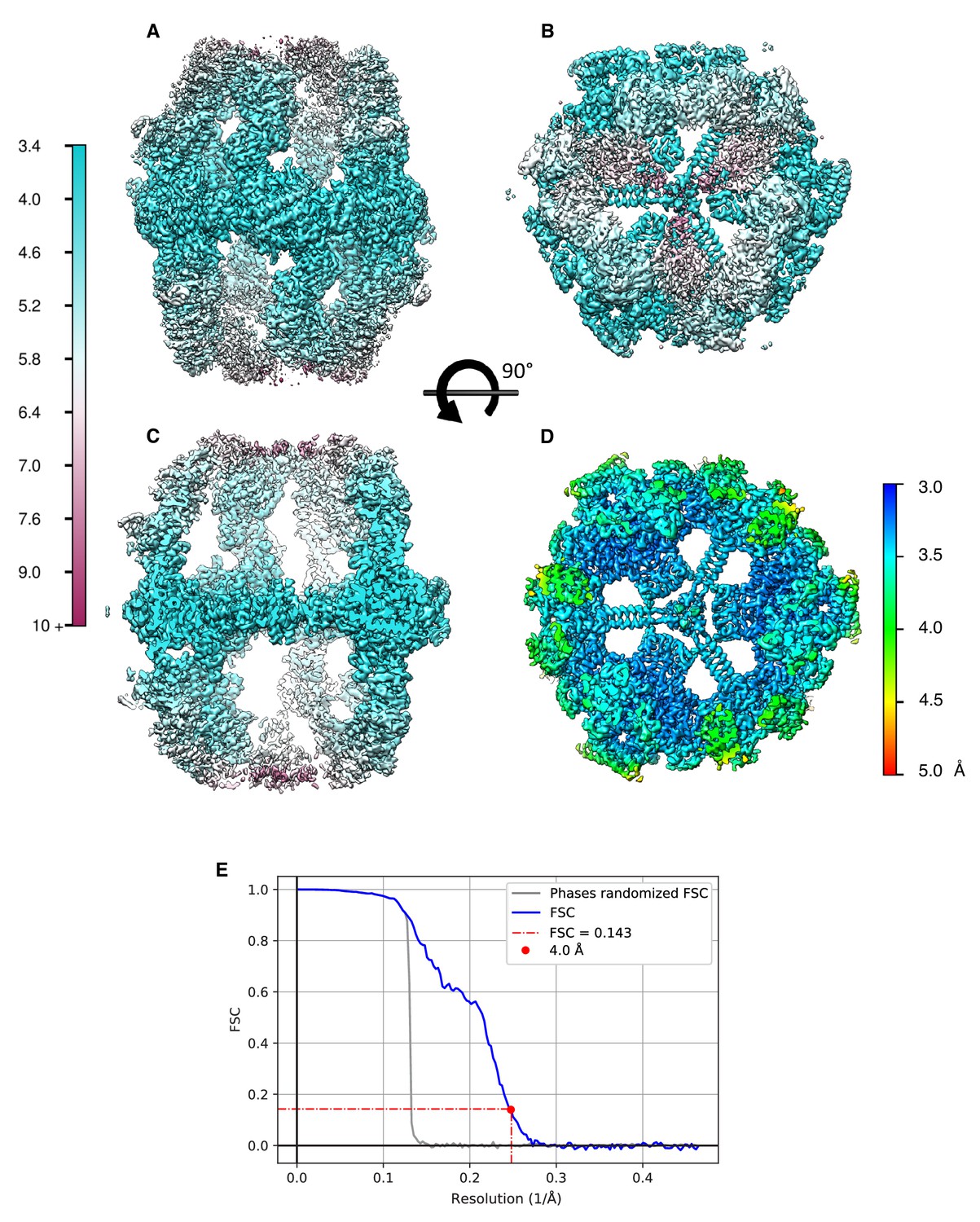
Local resolution estimates of FAS refined to a global resolution of 4.0 Å (Figure 6D) in side view.
(A) and top view (B). (C) Longitudinal section of (A). (D) Transversal section of (B) showing the central alpha wheel at a local resolution of 3.5 Å or better. (E) Fourier shell correlation of the half-maps, unfiltered (blue) and phase-randomized (grey).
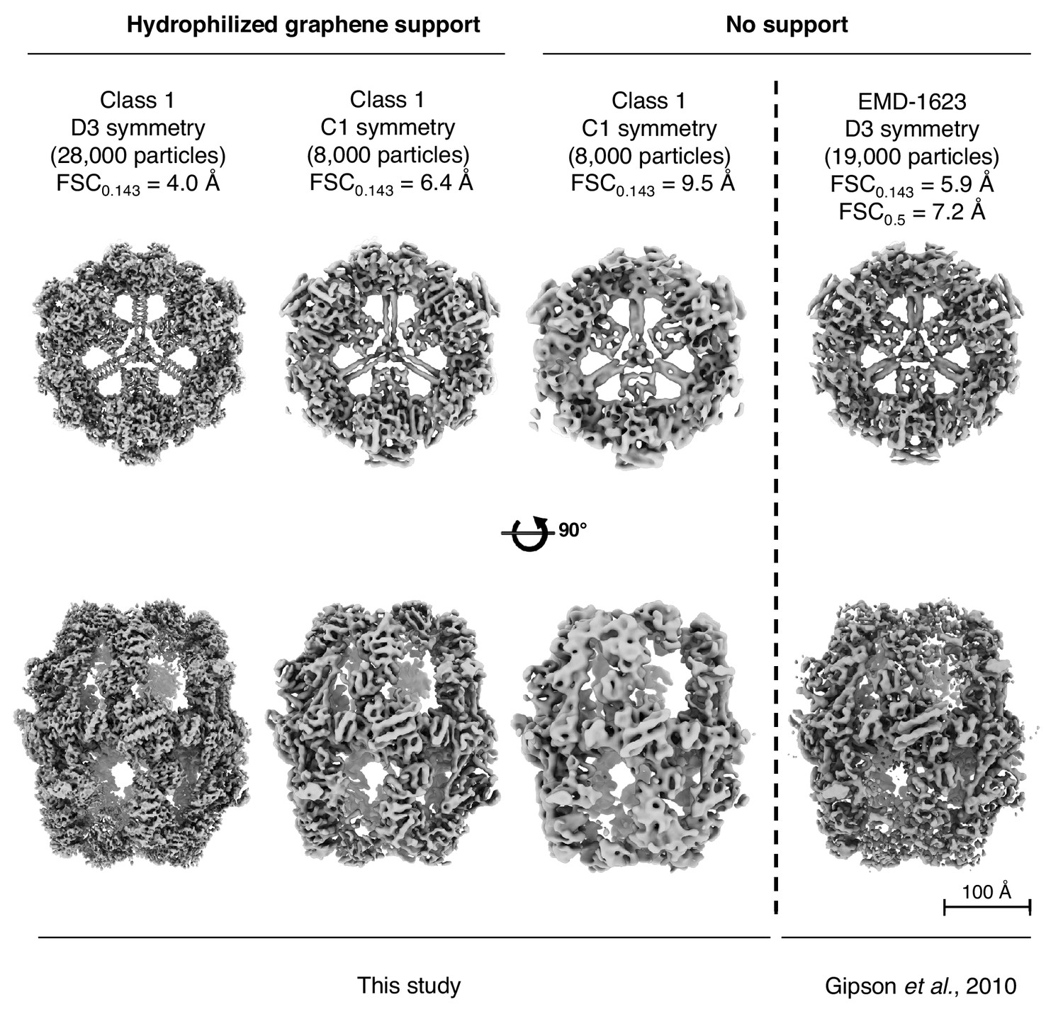
Figure 6—figure supplement 3
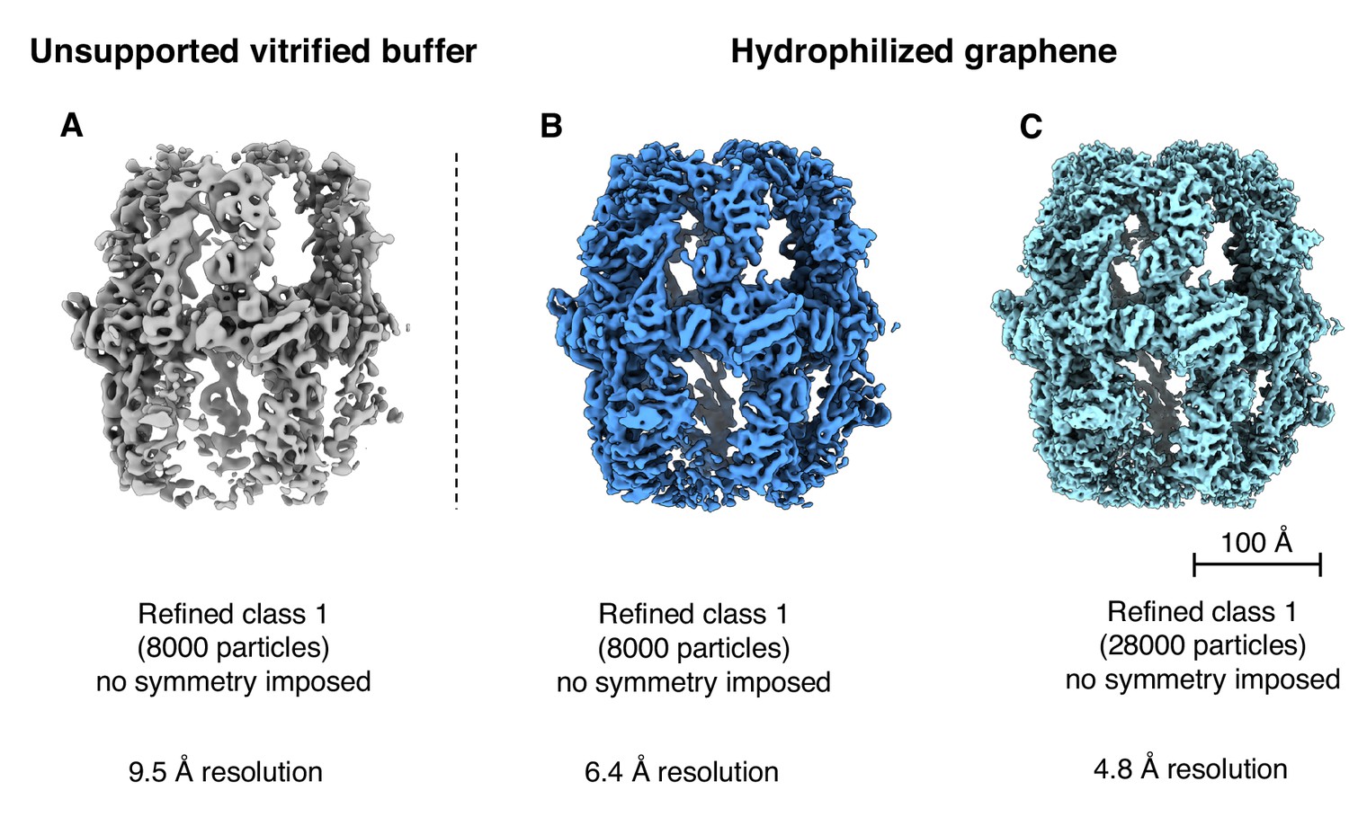
Reconstructions from different particle numbers.
(A) 8000 particles in unsupported vitrified buffer (Class one from Figure 1B); (B) 8000 particles from hydrophilized graphene supported samples; (C) 28,000 particles from hydrophilized graphene-supported samples (Class one from Figure 6B).
Figure 6—figure supplement 4
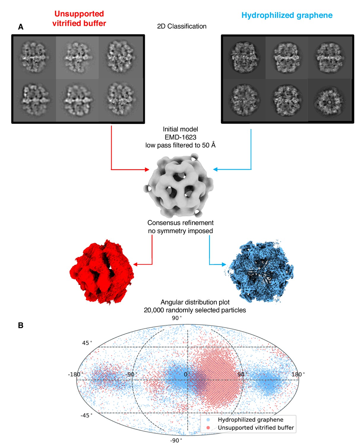
Particle orientation distribution.
(A) Overview of FAS map reconstruction after consensus refinement from the dataset on unsupported vitrified buffer and hydrophilized graphene respectively. (B) Angular distribution plot of equal subsets of particles after consensus refinement.
Figure 6—figure supplement 5
Comparison of cryo-EM maps obtained in this study to the published cryo-EM map of FAS (Gipson et al., 2010).
The resolution the published map (Gipson et al., 2010) is between our FAS reconstruction in unsupported vitrified buffer, and the reconstruction of FAS on hydrophilized graphene.
Additional files
-
Transparent reporting form
- https://doi.org/10.7554/eLife.42747.024
Download links
A two-part list of links to download the article, or parts of the article, in various formats.
Downloads (link to download the article as PDF)
Open citations (links to open the citations from this article in various online reference manager services)
Cite this article (links to download the citations from this article in formats compatible with various reference manager tools)
Protein denaturation at the air-water interface and how to prevent it
eLife 8:e42747.
https://doi.org/10.7554/eLife.42747


