HCN channel-mediated neuromodulation can control action potential velocity and fidelity in central axons
- University Leipzig, Germany
- Institute of Science and Technology Austria (IST Austria), Austria
- Max-Planck-Institute for Experimental Medicine, Germany
- Royal Netherlands Academy of Arts and Sciences, Netherlands
- University of Utrecht, Netherlands
Figures
Figure 1 with 1 supplement
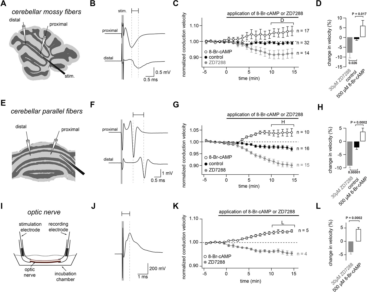
Bidirectional modulation of conduction velocity.
(A) Recording configuration of conduction velocity in mossy fibers using a bipolar tungsten stimulation electrode (stim.) and two glass recording electrodes. (B) Example of compound action potentials recorded with two electrodes positioned at different distances in relation to the stimulation electrode. The stimulation (100 µs duration) is indicated by the gray bar. Each trace is an average of 50 individual compound action potentials recorded at 1 Hz. The delay between the peak of the proximal and the distal compound action potential is indicated by a horizontal line. (C) Average normalized mossy fiber conduction velocity, during bath application (starting at t = 0 min)of ZD7288 (30 µM) or 8-Br-cAMP (500 µM). (D) Average relative changes in conduction velocity of mossy fiber measured 10 to 15 min after beginning the application of ZD7288 or 8-Br-cAMP (bracket in C). PANOVA = 0.00015. PKruskal-Wallis = 0.00044. The individual P values of the Dunnett test for multiple comparisons with the control are indicated. (E) Schematic illustration of the experimental configuration used to record from cerebellar parallel fibers. (F) Examples of compound action potentials recorded from parallel fibers, as in panel (B). (G) Normalized conduction velocity in parallel fibers, as in panel (C). (H) Average relative changes in conduction velocity parallel fibers, as in panel (D). PANOVA = 10−9. PKruskal-Wallis = 10−8. The individual P values of the Dunnett test for multiple comparisons with the control are indicated. (I) Schematic illustration of the experimental configuration used to record from optic nerve. (J) Examples of compound action potentials recorded from optic nerve, as in panel (B). (K) Normalized conduction velocity in optic nerve, as in panel (C). (L) Average relative changes in conduction velocity of optic nerve, as in panel (D). PT-Test = 0.0002. PWilcoxon-Mann-Whitney-Test = 0.004.
Figure 1—figure supplement 1
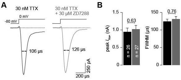
ZD7288 does not alter Na+ currents in cMFBs.
(A) Example whole-cell Na+ currents measured under control conditions (30 nM TTX) and in the presence of additional 30 µM ZD7288 elicited by voltage steps from –80 mV to 0 mV. (B) With 30 nM TTX present in the extracellular solution (see Materials and methods), the average Na+ current amplitude was 947.9 ± 107.5 pA (n = 26). In the presence of 30 nM TTX and 30 µM ZD7288, the amplitude did not differ from that of the currents recorded in 30 nM TTX only (1022.5 ± 109.0 pA; n = 27; PT-Test = 0.63). The average half-durations were 124.3 ± 6.2 µs and 131.5 ± 7.2 µs (PT-Test = 0.45) for control recordings and for recordings performed in the presence of 30 µM ZD7288, respectively.
Figure 2

Neuromodulators differentially regulate conduction velocity via HCN channels.
(A) Example of compound action potentials recorded in parallel fibers. Each trace is an average of signals recorded over a period of 1 min, before (at −5 min, black line) and after application of 200 µM NE (at 15 min, blue line). The delays between the peak of the proximal action potential and the distal compound action potential are indicated by horizontal bars. Traces are aligned to the peak of the compound action potentials recorded with the proximal electrode. (B) Example of compound action potentials as shown in panel (A) with the application of 200 µM adenosine. (C) Average normalized conduction velocity in cerebellar parallel fibers during the application of various neuromodulators that are known to act via cAMP-dependent pathways. (D) Average relative change in conduction velocity measured from 1 to 6 min after the start of neuromodulator application (bracket marked D in panel (C)). PANOVA = 9*10−10. PKruskal-Wallis = 3*10−8. The individual P values of the Dunnett test for multiple comparisons with the control are indicated. (E) Average relative change in conduction velocity measured from 10 to 15 min after the start of application of the neuromodulators (bracket marked E in panel (C)). PANOVA = 3*10−7. PKruskal-Wallis = 3*10−7. The individual P values of the Dunnett test for multiple comparisons with the control are indicated. (F) Average normalized conduction velocity in parallel fibers. 30 µM ZD7288 was applied 25 min before the start of the application of the neuromodulators. ZD7288 remained in the solution during recording to ensure continuously blocked HCN channels. At t = 0 min, 8-Br-cAMP, adenosine or NE was added to the solution. (G) Average relative change in conduction velocity measured 10 to 15 min after the start of application of the neuromodulators (bracket marked G in panel (F)). PANOVA = 0.91. PKruskal-Wallis = 0.77. The individual P values of the Dunnett test for multiple comparisons with the control are indicated.
Figure 3
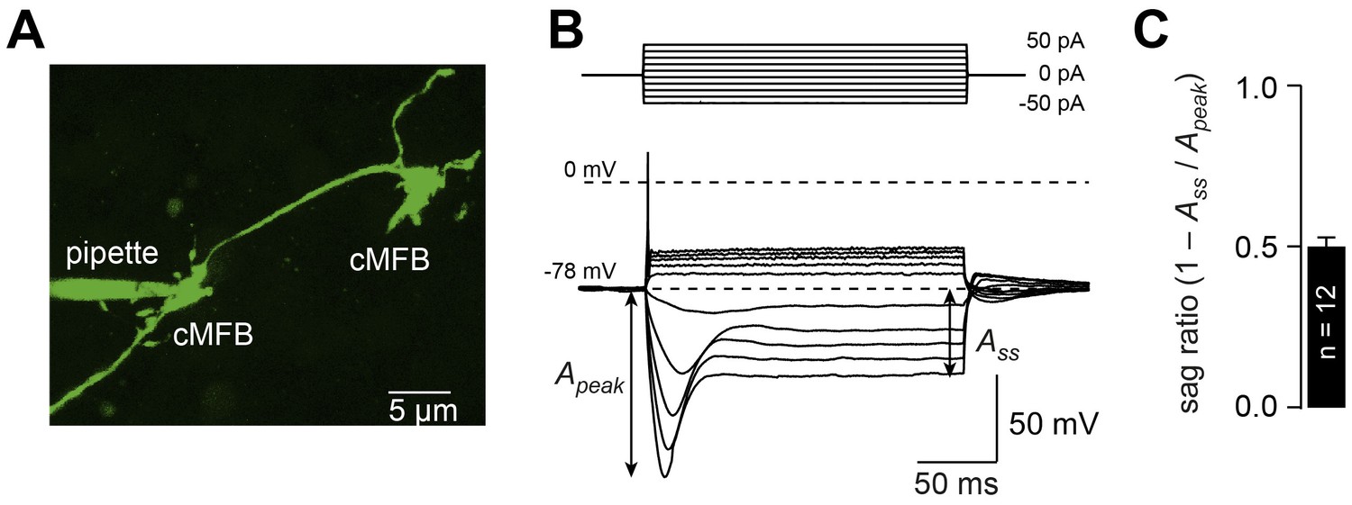
Cerebellar mossy fiber terminals have a prominent voltage sag.
(A) Two-photon microscopic image of a whole-cell patch-clamp recording from a cMFB (green) filled with the fluorescence dye Atto 488 in an acute cerebellar brain slice of an adult 39-day-old mouse (maximal projection of stack of images). (B) Characteristic response of a cMFB to current injection: depolarizing pulses evoked a single action potential and hyperpolarizing pulses evoked a strong hyperpolarization with a sag. (C) Average sag ratio of 12 cMFB recordings.
Figure 4
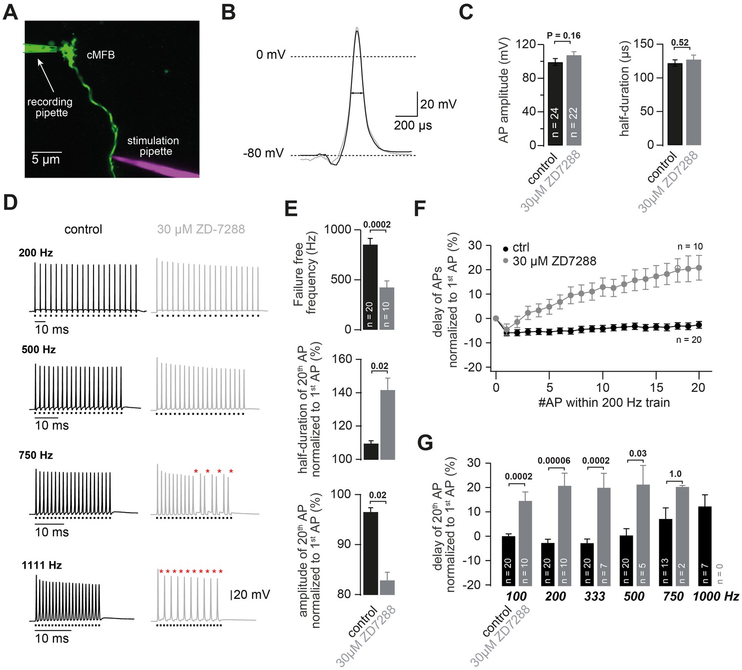
HCN channels support high-frequency action potential firing.
(A) Two-photon microscopic image of a whole-cell patch-clamp recording from a cMFB (green) filled with the fluorescent dye Atto 488 in an acute cerebellar brain slice of an adult (43-day-old) mouse (maximal projection of stack of images). Targeted axonal stimulation was performed by adding a red dye, Atto 594, to the solution of the stimulation pipette. (B) Grand average of action potentials evoked at 1 Hz under control conditions (black) and in the presence of ZD7288 (gray). (C) Average action potential amplitude (measured from resting to peak) and half-duration (PT-Test = 0.16 and 0.51 for amplitude and resting, respectively). (D) Example traces of two different cMFBs stimulated at frequencies between 200 Hz and 1111 Hz under control conditions (left, black) or in the presence of 30 µM ZD7288 (right, gray). Traces for 100, 333, 1000 and 1666 Hz are not shown. The time of stimulation is indicated below each trace. Failures are illustrated by red asterisks. (E) (Top graph) Average maximal failure-free firing frequency for control (black) and ZD7288-treated (gray) cMFBs. (Middle and bottom graph) Average amplitude reduction and action potential broadening of the 20th compared with the 1st action potential (AP) of trains of 20 stimuli at 200 Hz for control (black) and ZD7288-treated(gray) cMFBs. (F) Average delay between the peak of the APs and the stimulation during trains of 20 stimuli at 200 Hz, normalized to the delay of the first AP, for control conditions (black) and ZD7288-treated (gray) cMFBs. (G) Average delay of the 20th AP normalized to the delay of the 1staction potential during failure-free trains of 20 stimuli at frequencies ranging from 100 to 1000 Hz. The P-values were obtained from t-tests and were multiplied by six to apply a Bonferroni-correction, indicating a highly significant slowing of the conduction velocity during failure-free high-frequency trains in ZD7288-treated cMFBs compared with controls. Note that the number of experiments decreased with increasing frequency because the analysis harestricted to failure-free traces.
Figure 5
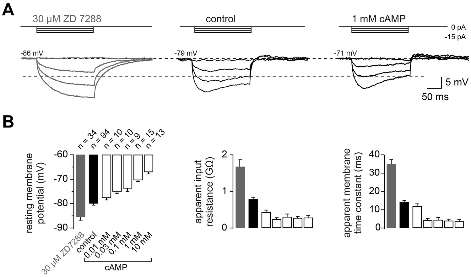
The passive membrane properties of cMFBs are HCN- and cAMP-dependent.
(A) Example voltage response of cMFBs to small hyperpolarizing current steps. The application of 30 µM ZD7288 eliminated the Ih-mediated voltage sag (left). Adding 1 mM cAMP to the intracellular path-clamp solution (right) reduced the input resistance as seen by the reduced steady-state voltage response (dashed lines). (B) Average resting membrane potential (left), apparent input resistance (middle), and apparent membrane time constant (right) upon application of 30 µM ZD7288 or different concentrations of cAMP. For all three parameters, PANOVA and PKruskal-Wallis are <10−10. The Dunnett test for multiple comparisons with the control indicates significance for control vs. ZD7288 (p<0.0001) and for control vs. cAMP concentrations >~0.1 mM (e.g., P<0.001 for control vs. 1 mM cAMP).
Figure 6 with 1 supplement
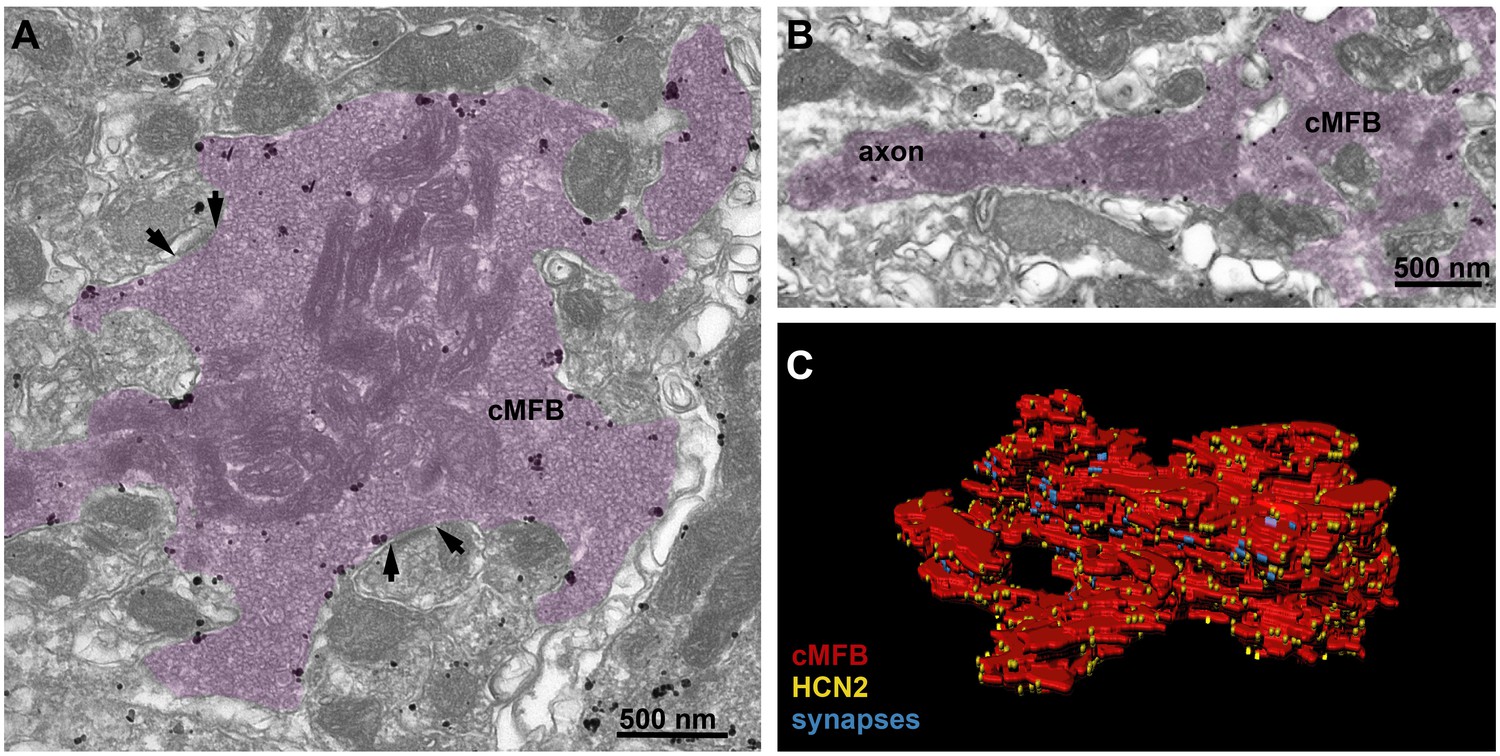
HCN2 is uniformly distributed in mossy fiber axons and boutons.
(A) Electron microscopic image showing a cMFB (magenta) labeled for HCN2. Many particles are diffusely distributed along the plasma membrane of the cMFB, some of them being clustered. Arrows mark synapses between the cMFB and dendrites of adjacent granule cells. (B) Another cMFB, showing similar labeling density for HCN2 in a proximal part of the mossy fiber axon. (C) Reconstructed cMFB (red) with identified synapses based on the ultrastructure (blue) and with HCN2 labeled with gold particles (yellow).
Figure 6—video 1
Reconstructed cMFB with labeled synapses and HCN2 channels.
3D rendering of a part of a reconstructed cMFB (red) with identified synapses (blue) and HCN2 labeled with gold particles (yellow) based on immune-gold electron microscopic images.
Figure 7
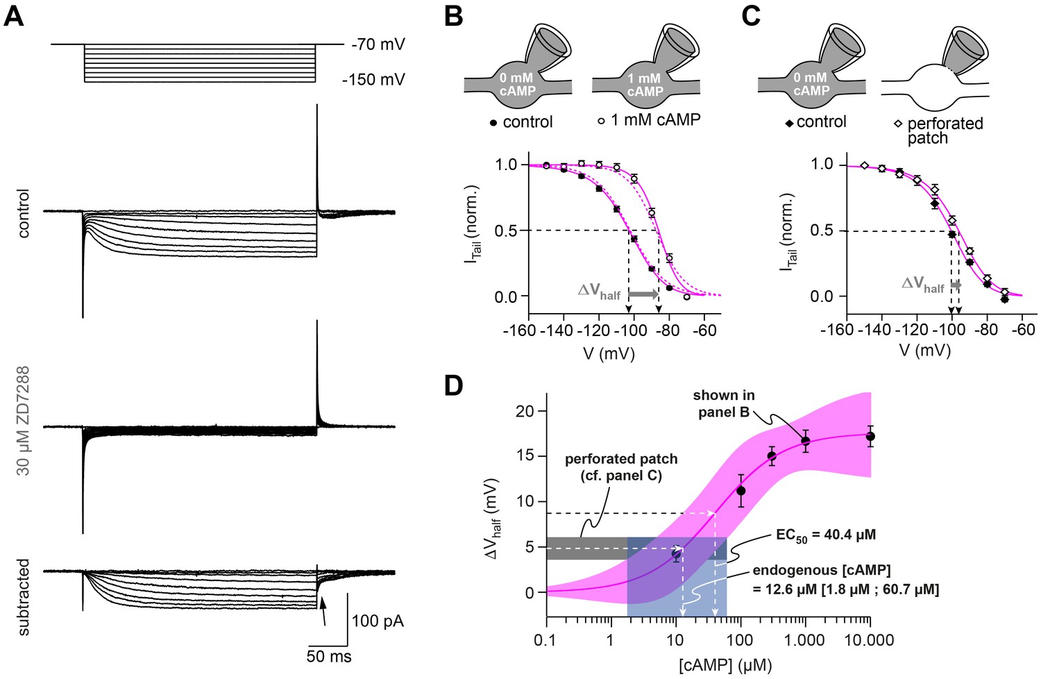
HCN channels in cMFB are strongly modulated by cAMP.
(A) Example currents elicited by hyperpolarizing voltage steps (from –70 mV to a voltage between –70 mV and –150 mV). Top, control current, middle, remaining transients in the presence of 30 µM ZD7288 and, bottom, subtracted currents. The ZD7288-sensitive current is slowly activating, non-inactivating and shows inward tail currents (arrow). (B) Activation curve of Ih determined as the normalized tail current of ZD7288-sensitive currents obtained after the end of the conditioning voltage pulse (arrow in panel (A)) plotted against the corresponding voltage pulse with 0 mM cAMP (filled circles, n = 36) and 1 mM cAMP (open circles, n = 15) in the intracellular solution. Sigmoidal fits (continuous magenta lines) yield the midpoints of Ih activation (V½, arrows). The steady-state activation curves produced by the Hodgkin-Huxley models (dotted magenta line) are superimposed. Inset on top: illustration of the whole-cell recording configuration with 0 and 1 mM cAMP in the intracellular solution. (C) Activation curves obtained with the perforated-patch recordings and after rupture of the perforated membrane patch (n = 10). Inset on top: illustration of the whole-cell recording configuration with 0 mM cAMP in the intracellular solution and in the perforated patch configuration, when the intracellular cAMP concentration is unperturbed. (D) Shift in Ih V½ versus the corresponding cAMP concentration (mean ± SEM). Fitting the data with a Hill equation (magenta line) revealed an EC50 of 40.4 µM. Superposition of the 68% confidence band of the fit (light magenta area) with the average voltage shift observed in perforated patch recordings (4.8 ± 1.2 mV, n = 10, dotted black line and gray area) results in an estimated endogenous cAMP-concentration of 12.6 µM with a 68% confidence interval of 1.8 to 60.7 µM cAMP (dotted line and light blue area).
Figure 8
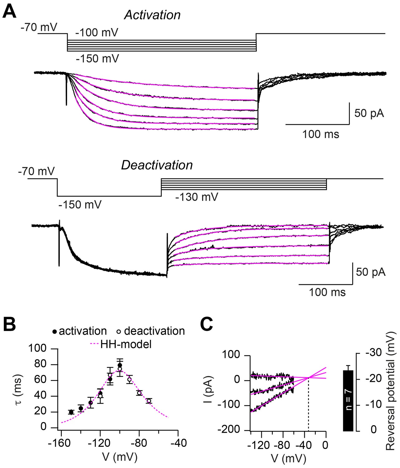
Hodgkin-Huxley model describing HCN2 channel gating.
(A) Example of ZD7288-sensitive currents (black) elicited by the illustrated activation (top) and deactivation (bottom) voltage protocols superimposed with mono-exponential fits (magenta). (B) Average time constants of activation (filled circles) and deactivation (open circles; mean ± SEM). The dotted magenta line represents the prediction of Ih activation and deactivation time constant based on the Hodgkin-Huxley model. (C) Example of linear extrapolation (magenta lines) of leak subtracted currents evoked by fast (10 ms) voltage ramps generated from a range of holding potentials that extended across the activation range of Ih. The reversal potential was found to be –36 mV in this example. Inset: average reversal potential from seven independent experiments.
Figure 9 with 1 supplement
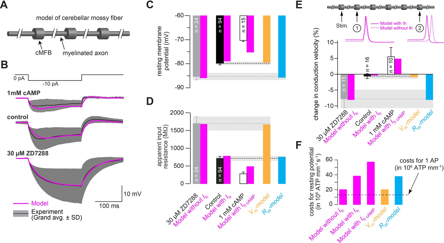
Mechanism of control of conduction velocity and metabolic costs of HCN channels.
(A) Illustration of the cerebellar mossy fiber model consisting of 15 connected cylindrical compartments representing cMFBs and the myelinated axon. (B) Grand average voltage response (black) and standard deviation (gray area) of cMFBs to a –10 pA hyperpolarizing current pulse with 1 mM cAMP included in the patch pipette (top), under control conditions (middle) or for cMFBs treated with ZD7288 (bottom), superimposed with the predicted voltage response from the model (magenta). (C) Average resting membrane potential of cMFBs measured under control conditions (black), with ZD7288 (gray), or 1 mM intracellular cAMP (open bar; data from Figure 5B) compared to the predictions from the corresponding models (magenta). Furthermore, the chart also shows the resting membrane potential of the two models that simulate only the membrane depolarization (Vm- model; light brown) or only the decreased membrane resistance (Rm-model; blue) caused by HCN channels. (D) Corresponding comparison between the measured values and the predictions from the models as shown in panel (C) for the apparent input resistance of cMFBs. (E) Corresponding comparison between the measured values and the predictions from the models as shown in panels (C) and (D) for the conduction velocity in mossy fibers. Inset top: illustration of the model of a mossy fiber and the action potentials at two different positions with (magenta line) and without (dashed magenta line) the HH model of HCN channels. (F) The calculated metabolic costs for maintaining the resting membrane potential are shown for each model as the number of required ATP molecules per mm of mossy fiber axon and per second. The metabolic cost of the firing of a single action potential (AP) is indicated by the dashed line as the number of required ATP molecules per mm of mossy fiber axon (this number was very similar for all models).
Figure 9—figure supplement 1
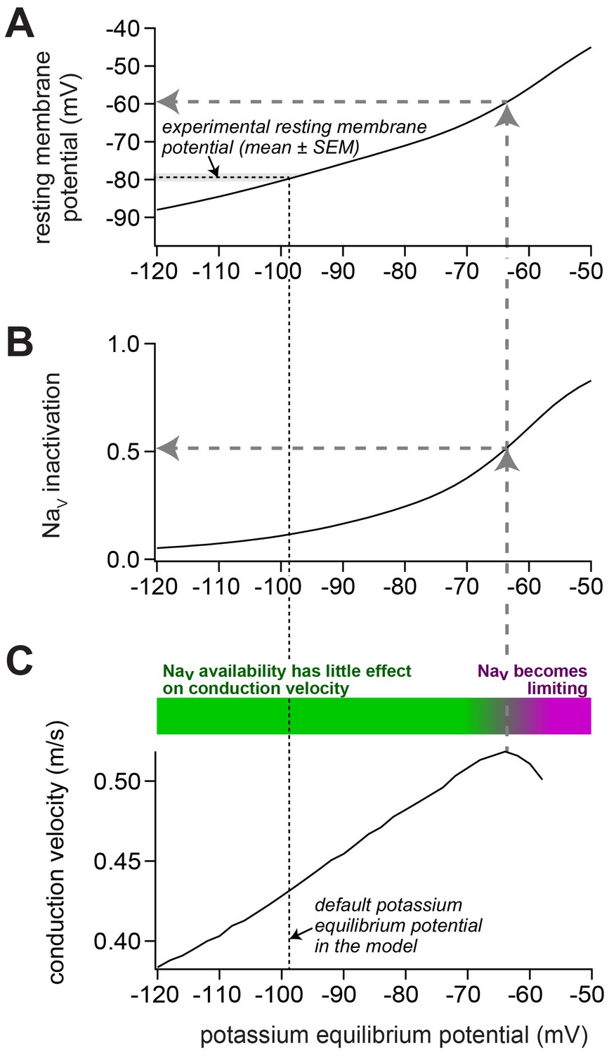
Impact of depolarization on NaV availability and on conduction velocity in our model of a mossy fiber axon.
(A) To change the resting membrane potential, the potassium equilibrium potential was varied between –120 and –50 mV. In the default model, the experimentally observed resting membrane potential (indicated by the horizontal black dashed line and the gray bar; mean ± SEM) was obtained with a potassium equilibrium potential of –98 mV (vertical black dashed line). (B) Upon depolarization, the inactivation of voltage-dependent sodium (NaV) channels increased. For the control model, the NaV inactivation was 12%. For the model reproducing the experiments with ZD7288 and 1 mM intracellular cAMP, the NaV inactivation was 6% and 17%, respectively. Because the steady-state NaV availability depends mostly on the resting membrane potential, the relation between resting membrane potential and NaV availability was identical for all three models (data not shown). (C) Upon depolarization, the conduction velocity increased up to a potassium equilibrium potential of about –65 mV (vertical gray dashed arrow), corresponding to an NaV availability of about 50% (horizontal gray dashed arrow in panel (B)) and a resting membrane potential of about –60 mV (horizontal gray dashed arrow in panel (A)). Thus, despite increasing NaV inactivation, the conduction velocity increased in this range (as illustrated by the green bar). With stronger depolarization, the conduction velocity declined, indicating that the NaV availability becomes limiting for conduction velocity (purple bar).
Additional files
-
Transparent reporting form
- https://doi.org/10.7554/eLife.42766.014
Download links
A two-part list of links to download the article, or parts of the article, in various formats.
Downloads (link to download the article as PDF)
Open citations (links to open the citations from this article in various online reference manager services)
Cite this article (links to download the citations from this article in formats compatible with various reference manager tools)
HCN channel-mediated neuromodulation can control action potential velocity and fidelity in central axons
eLife 8:e42766.
https://doi.org/10.7554/eLife.42766


