Visual cue-related activity of cells in the medial entorhinal cortex during navigation in virtual reality
- Princeton Neuroscience Institute, Princeton University, United States
- Bezos Center for Neural Circuit Dynamics, Princeton University, United States
- Department of Molecular Biology, Princeton University, United States
Figures
Figure 1 with 3 supplements
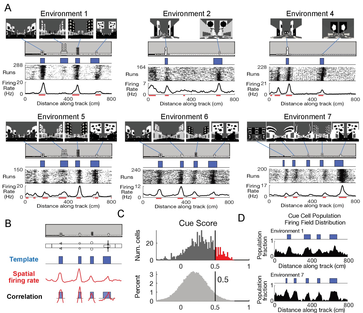
Cells respond to cues in a virtual linear environment.
(A) Examples of cells with cue-related activity recorded during navigation along virtual tracks. At the top of each example are views of each cue from the animal’s perspective inside the track at that location. Side views of the track are shown below, with the start location to the left. The raster plot for a single cell’s spatial activity pattern across multiple traversals of the track is plotted with the average firing rate (Hz) as a function of track position (spatial firing rate) below. Spatial firing fields for the cell are indicated with horizontal red bars. (B) Calculation of cue score. The Pearson correlation between the cue template and the cell’s spatial firing rate was calculated and the spatial shift was defined as the local maximum closest to zero. The cue template was translated by this shift and the correlations of this shifted cue template and spatial firing rate at each cue were individually calculated. The cue score was defined to be the mean of these correlations (Materials and Methods). (C) The distribution of cue scores of recorded cells is shown at the top with the distribution of cue scores calculated on shuffled data shown below. The threshold was chosen as the value that 95% of the shuffled scores did not exceed (vertical black line). Cells exceeding this threshold were termed ‘cue cells’ and are shown in red in the top plot. (D) Distribution of spatial firing fields of all cue cells in two environments.
-
Figure 1—source data 1
Cue score and shuffle distributions.
- https://cdn.elifesciences.org/articles/43140/elife-43140-fig1-data1-v2.mat
-
Figure 1—source data 2
Cue cell population field distributions across the virtual tracks.
- https://cdn.elifesciences.org/articles/43140/elife-43140-fig1-data2-v2.mat
Figure 1—figure supplement 1
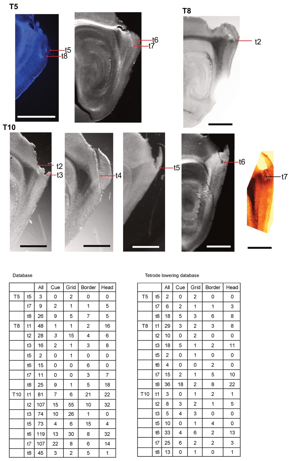
Histology of tetrode tracks and tetrode cell type summary.
All images were sharpened and recolored to emphasize tetrode tracks and lesions. Scale bar = 1 mm. Tables show summaries of cell types for each animal for the database used in the main figures and for the database shown in the figure supplements (tetrode lowering database).
Figure 1—figure supplement 2
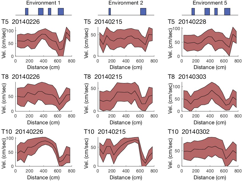
Velocity profiles of navigation along virtual tracks.
Examples of the mean ± standard deviation velocity profiles of animals running along 3 different virtual tracks.
Figure 1—figure supplement 3

Cue cells in tetrode lowering database.
Summary plots for a database including only dates in which tetrodes were lowered (tetrode lowering database). Cue cells accounted for 19% of cells in this database. The mean firing field fraction for spatial bins of the firing field distribution in cue regions (0.40 ± 0.14) was higher than that for bins outside of cue regions (0.26 ± 0.18) (paired one-tailed t-test: cell fraction in cue regions > cell fraction outside cue regions, N = 52, p=4 × 10⁻⁷).
Figure 2 with 2 supplements
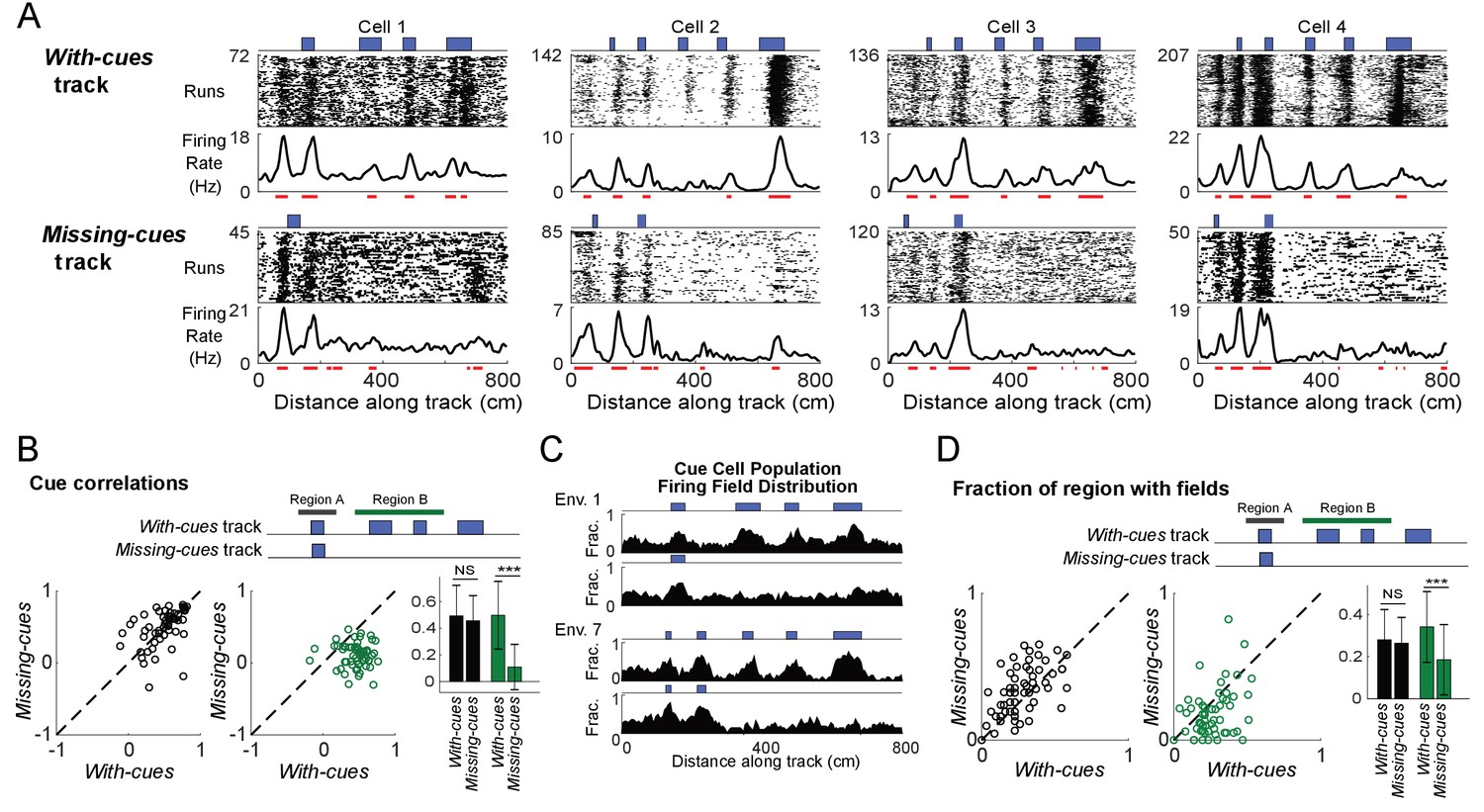
Cells respond to cue changes in an environment.
(A) Examples of the spatial firing rates of cells during cue perturbation experiments. For each example, the top and bottom panels are from the same cell in blocks of trials in which the animal either ran down a virtual track with all cues present (with-cues track, top) or a track where some cues were missing in the later part of the track (missing-cues track, bottom). The environment and cue template for both environments are shown with the corresponding raster plots and spatial firing rates below. (B) Cue correlations of the firing rates along the with-cues and missing cues tracks within Regions A and B were calculated. The correlation of firing rate to cue was lower for the firing rates on the missing cues track in Region B (paired one-tailed t-test: cue correlation on with-cues track >cue correlation on missing-cues track, N = 65, 3 animals, for Region A, p=0.56, for Region B, p=1×10⁻¹⁴). On the right, the means with standard deviations are shown for regions A and B on each track. (C) Population field distribution for the entire population of cue cells along with-cues and missing-cues tracks for two environments. (D) Comparison of firing fields of all cue cells between runs in the initial region that is the same for both tracks (Region A) and the later region (Region B) on the with-cues and missing-cues tracks. The fraction of each region that had spatial firing fields (number of field bins/total bins in that region) is plotted for each cue cell. The field fraction was larger in region B on the with-cues track in comparison to region B on the missing-cues track (paired one-tailed t-test: field fraction on with-cues track >cue field fraction on missing-cues track, N = 65, 3 animals, for region A: p=1.00, for region B, p=0.0002). On the right, the means with standard deviations are shown for regions A and B on each track. ***p≤0.001. Student’s t-test.
-
Figure 2—source data 1
Cue cell firing field fractions.
- https://cdn.elifesciences.org/articles/43140/elife-43140-fig2-data1-v2.mat
-
Figure 2—source data 2
Correlations of firing rates along tracks to cue template.
- https://cdn.elifesciences.org/articles/43140/elife-43140-fig2-data2-v2.mat
Figure 2—figure supplement 1

Cue-removal responses of cue cells with fields near or far from cues.
Data shown in Figure 2 is separated into subgroups based on the spatial shift of the firing rate of each cue cell relative to the cue template. Plots from Figure 2B–D are shown for each group. Cells with spatial shifts less than and more than 25 cm in either direction were categorized as cells with fields near and far from cues, respectively. Top panel stats: Cue cells with fields near cues. For cue correlations: Region A, p=0.95; Region B, p=6×10⁻¹⁴. For fractions of regions with fields: Region A, p=0.99; Region B, p=0.004. Bottom panel stats: Cue cells with fields far from cues. For cue correlations: Region A, p=0.16; Region B, p=0.004. For fractions of regions with fields: Region A, p=0.98; Region B, p=0.004. ***p≤0.001. **p≤0.005 Student’s t-test.
Figure 2—figure supplement 2

Cue cell responses to cue changes for tetrode lowering database.
Statistics for Figure 2 plots using the tetrode lowering database. For cue correlations: Region A, p=0.66; Region B, p=4×10⁻¹⁰. For fractions of regions with fields: Region A, p=1.00; Region B, p=0.03. ***p≤0.001. *p≤0.05 Student’s t-test.
Figure 3 with 2 supplements
Cue cell activity during foraging in a real arena.
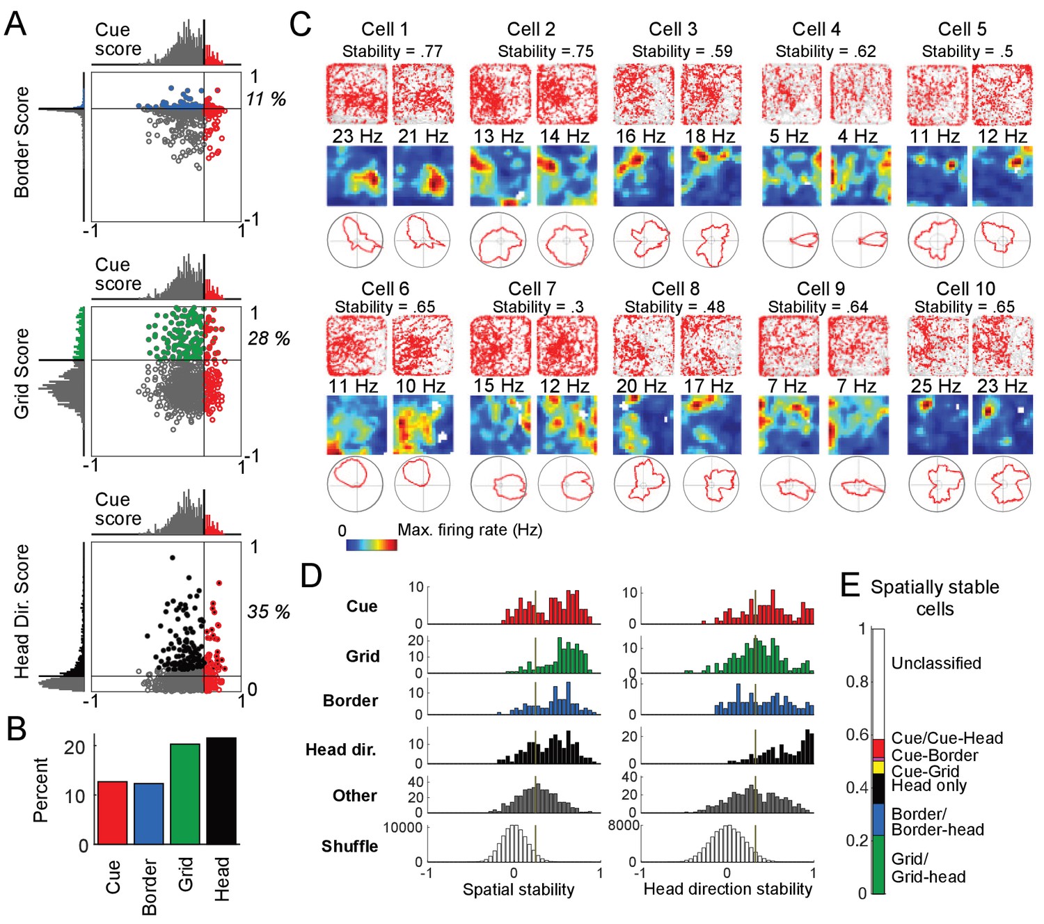
(A) Relative distributions of cue scores compared to border, grid, and head direction scores. Thresholds were calculated as the value that exceeds 95% of the shuffled scores. The solid line indicates the threshold for each score that was used to determine the corresponding cell type (Materials and Methods). Cells are color-coded for whether they are cue (red), grid (green), border (blue), or head direction cells (black). The percentage of the cue cell population that was conjunctive for border, grid, and head direction is shown in each plot. (B) Percentage of each cell type in the dataset. (C) Examples of the spatial stability of the spatial firing rates of cue cells in a real arena. The recording of each cell was divided in half. The spatial firing rates of the first and second halves are shown for each cell in the left and right columns. Within each column: top: plots of spike locations (red dots) and trajectory (gray lines); middle: the 2D spatial firing rate (represented in a heat map with the maximum firing rate indicated above); bottom: head direction firing rate. The stability was calculated as the correlation of these two firing rates and shown at the top for each cell. (D) Histograms of the spatial and head direction stability of the 2D real environment firing rates by cell type. (E) Percentage of 2D real environment stable cells that are of a certain type. Cell types are color-coded: red = cue cell, green = grid cell, blue = border cell, black = head direction cell.
-
Figure 3—source data 1
Cue, border, grid and head direction scores.
- https://cdn.elifesciences.org/articles/43140/elife-43140-fig3-data1-v2.mat
-
Figure 3—source data 2
Spatial and head direction stability values by cell type.
- https://cdn.elifesciences.org/articles/43140/elife-43140-fig3-data2-v2.mat
Figure 3—figure supplement 1
Cue cell activity in real arenas.
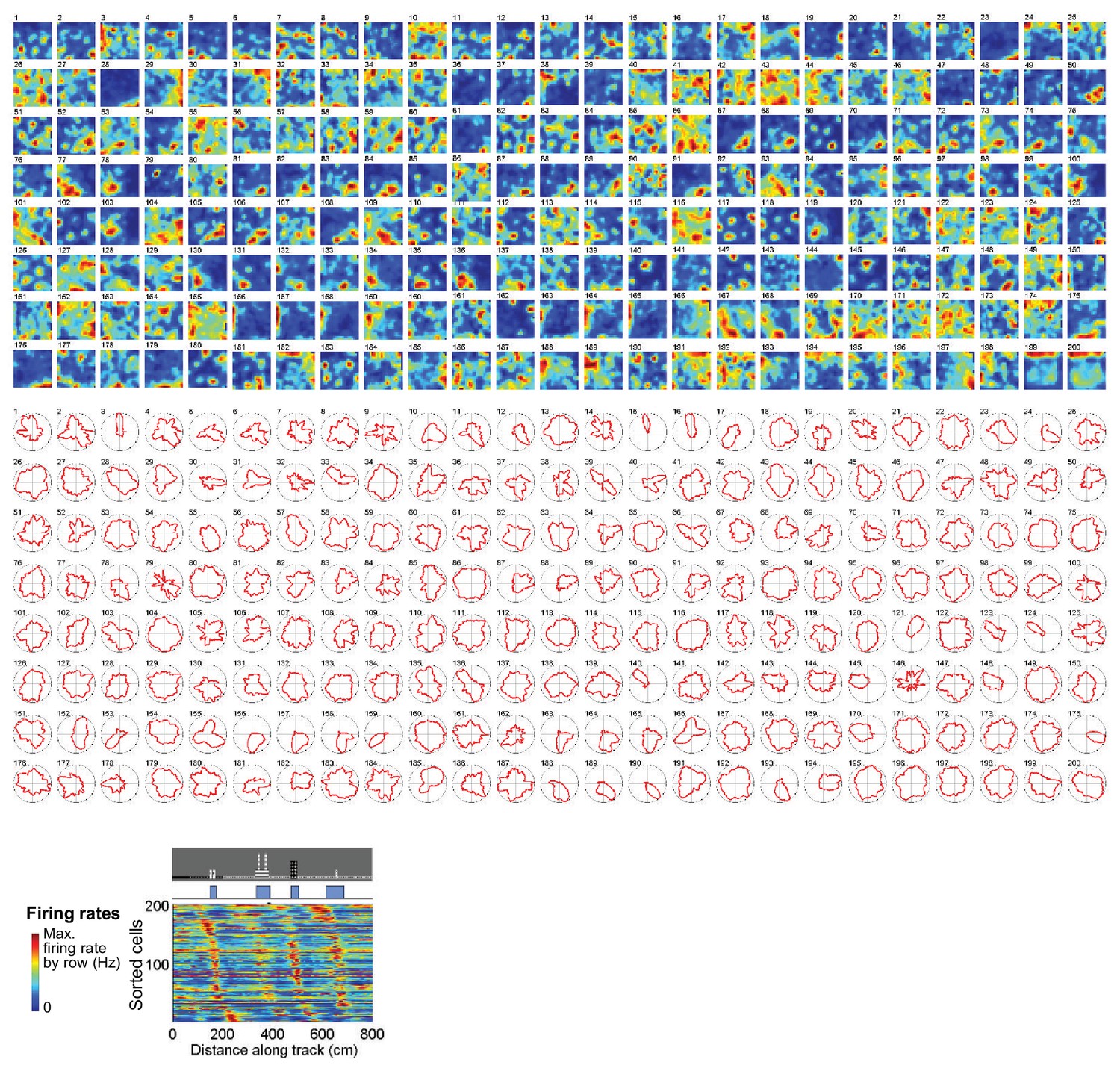
Top and middle panels: the spatial and head direction firing rates of cue cells in a real arena are sorted based on the spatial shifts of their spatial firing fields to the cue template in virtual reality (bottom panel). No clear patterns of changes in number, size and location of firing fields or the mean vector length of head direction firing rates were observed. In most cases, the cue card was located on the right wall of the environment.
Figure 3—figure supplement 2

Real arena navigation for tetrode lowering database.
Summary of cell type percentages and distributions for database including days when tetrodes were lowered.
Figure 4 with 1 supplement
Cue cells form a sequence aligned at each cue.
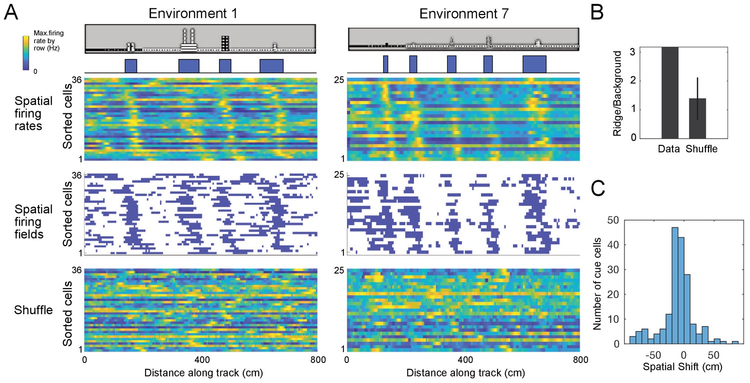
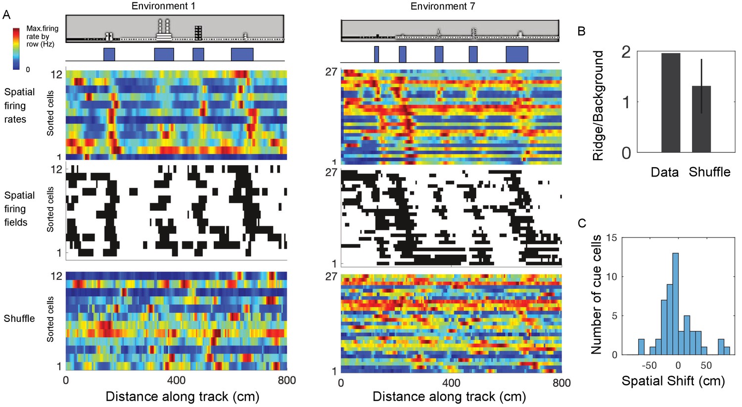
(A) Cue cell sequences shown for two environments. Top two rows show a side view of the virtual track and the corresponding cue template below. Just below this, the spatial firing rates, where the normalized firing rate of a cue cell is plotted along each row is shown. The cells are sorted based on their spatial shifts calculated for alignment of spatial firing rates to the cue template (Materials and Methods). The corresponding spatial firing fields of the same cells above are shown in the middle panel with the firing fields ordered in the same sequence as the firing rates. At the bottom, an example of the sorted shuffled spatial firing rates which were generated by shuffling the firing fields of each cell and then sorting based on their spatial shifts to the cue templates. (B) The ridge to background ratio for the data and shuffles of environment 1. (C) Distribution of spatial shifts for all cue cells.
-
Figure 4—source data 1
Cue cell sequences.
- https://cdn.elifesciences.org/articles/43140/elife-43140-fig4-data1-v2.mat
Figure 4—figure supplement 1
Cue cell sequences in tetrode lowering database.
Figure 5 with 5 supplements

Cue cell responses to side-specific cues in layer 2 of the MEC.
(A) A 1000 cm (10 meter) long virtual linear track for imaging experiments. ‘L’ and ‘R’ indicate cues on the left and right sides of the track, respectively. (B) Left and right cue templates with cues on the left and right sides of the track. (C) Examples of individual cue cells responding to the left- (top) or right-side cues (bottom) in layer 2 of the MEC. For each cell: top: ΔF/F versus linear track position for a set of sequential traversals. Middle: mean ΔF/F versus linear track position. Bottom: overlay of the cue template and aligned mean ΔF/F (black) according to the spatial shift, which gave the highest correlation between them (Materials and Methods). (D) Left and right cue cell sequences aligned to left- (top) and right-side cues (bottom), respectively. In each row the mean ΔF/F of a single cell along the track, normalized by its maximum, is plotted. The cells are sorted by the spatial shifts identified from the correlationof their mean ΔF/F to the cue template. (E) Bilateral scores of all left and right cells in D. Left: bilateral scores of individual cells (dots). Right: kernel density distribution of bilateral scores. Note that the bilateral scores show a strong bimodal distribution. (F) Percentages of cue cells among all cells activeduring virtual navigation (active cells were determined as cells identified using independent component analysis, Materials and Methods) . Left bar: all left and right cue cells. Middle bar: left cue cells. Right bar: right cue cells. Individual data points that were pooled for this are the percentages of cue cells in 12 FOVs in layer 2, p=6.90 × 10⁻⁴. (G) Comparison of cue scores of left and right cue cells in layer 2. Individual data points are cue scores of cells in D,p=1.67 × 10⁻⁵. All data were generated using layer 2 cue cells in 12 FOVs in four mice. ***p≤0.001. Student’s t-test.
-
Figure 5—source data 1
Cue scores, bilateral scores and percentages of left and right cue cells.
- https://cdn.elifesciences.org/articles/43140/elife-43140-fig5-data1-v2.mat
Figure 5—figure supplement 1
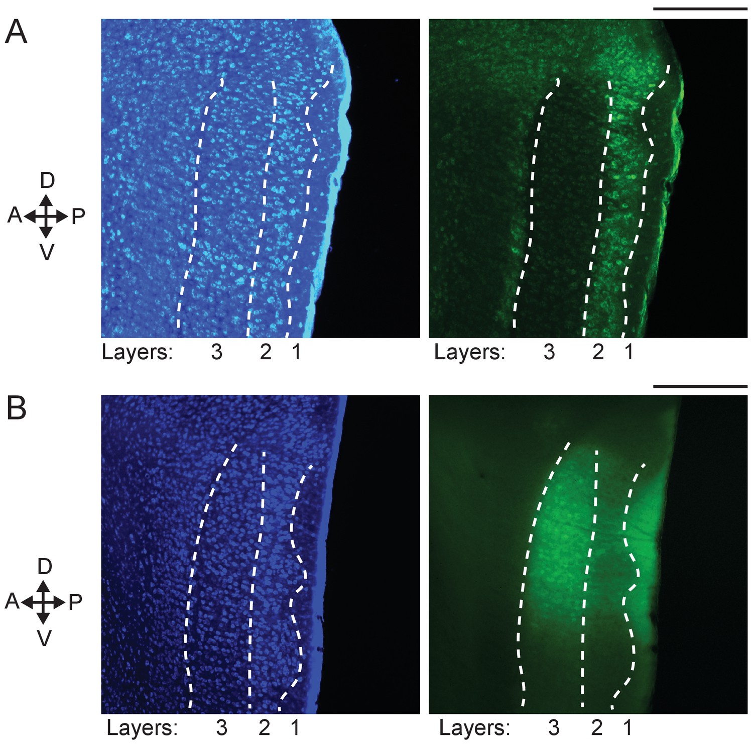
Expression of GCaMP6f in layers 2 and 3 of the mouse MEC.
(A) Expression of GCaMP6f in layer 2 of the MEC, shown with an image of a sagittal brain slice of a GP5.3 mouse at 5 months of age. Left: blue epifluorescence image showing cell bodies in layers 2 and 3 (separately delineated by white dotted curves) of the MEC labeled by fluorescent Nissl staining. Right: green epifluorescence image of the same slice on the left showing GCaMP6f expression of layer 2 neurons in the MEC. Scale bar: 200 µm. (B) Expression of GCaMP6f in layer 3 of the MEC, shown with an image of a sagittal brain slice of a wild type mouse 13 days after the injection of AAV1-hSyn-GCaMP6f virus in the MEC. Left: blue epifluorescence image showing cell bodies in layers 2 and 3 (boundaries shown by white dotted curves) of the MEC labeled by fluorescent Nissl staining. Right: green epifluorescence image of the same slice on the left showing GCaMP6f expression of dorsal layer 3 neurons in the MEC. Scale bar: 200 µm. The results of the imaged layer 3 cells are shown in Figure 5—figure supplement 4.
Figure 5—figure supplement 2

Cue cells preferentially represent cues on a single side, rather than both sides of the track.
(A) Left and right cue scores in layer 2 of the MEC. The locations of each circle/dot on the x and y axes represent the right and left cue scores for a cell, respectively. The solid line indicates the threshold for each type of score that was used to determine the corresponding cue cell type. Cells are color-coded according to whether they were right cue cells (magenta circles), left cue cells (green dots), or cells with cue scores that exceeded both right and left cue score thresholds (green dots with magenta outline). The scores of cells below all thresholds are shown as gray circles. The distributions of right and left scores are shown on the top and left of the plots with corresponding colors indicating cue scores above thresholds. (B) Spatial shifts on left and right templates for the 14 layer 2 cue cells (from 12 FOVs in four mice) that passed the thresholds of both templates. Each dot represents one cell. The bigger dot contains two data points with identical x and y coordinates. The gray dotted line indicates x = y. (C–G) Cue cells classified using the both-side cue template, which included cues on both left and right sides of the track. We classified cells using a threshold specific to the both-side template (B). However, we concluded that the cues on both sides were not well represented by the classified cells based on the following three reasons: 1.) The cue scores of both-side cue cells were significantly lower than those of left and right cue cells (D). Since the cue score is defined to be the mean correlation of a cell's response to individual cues, independent of the number of cues on a template, the low cue scores indicate that the responses of both-side cue cells did not correlate well to cues on both sides of the track. 2.) 64% of both-side cue cells were also classified as left or right cue cells, which only strongly responded to cues on one side (E, cell examples in F and G, the first and second panels). 3.) The rest of both-side cue cells (36%) only weakly correlated to the both-side template (E, cell examples in F and G, the third panels), as reflected by their lower cue scores (D). Cue cell sequences aligned to both-side cue template (top). Each row is mean ΔF/F of a single cell along the track, normalized by its maximum. The cells are sorted by the spatial shifts of their mean ΔF/F to the both-side cue template. (D) Comparison of cue scores. From left to right: scores of cells that passed the threshold of left, right, and both-side templates. Among the both-side cue cells, from left to right: all both-side cue cells; both-side cue cells that also independently had left and right cue scores that exceeded the thresholds for those scores; both-side cue cells that were not classified as left and right cue cells (non-left/non-right cells). p value: column 1 to 3: 4.35 × 10−37. Column 2 to 3: 4.08 × 10−63. Column 4 to 5: 7.16 × 10⁻⁴. (E) Pie chart showing the percentage of both-side cue cells that were also classified as left and right cue cells (white) and non-left and non-right cue cells (gray). (F) Three examples of both-side cue cells. Left: a both-side cue cell that is also identified as a left cue cell; middle: same but for a right cue cell; Right: a cell uniquely identified as a both-side cue cell (non-left/non-right cue cells). For each cell: top: ΔF/F versus linear track position for a set of sequential traversals. Middle: mean ΔF/F versus linear track position. Bottom: overlay of the cue template and aligned mean ΔF/F (black) according to the spatial shift. The left (green) and right cues (magenta) in the both-side cue templates are also shown in corresponding colors. (G) Cue cell sequences of both-side cue cells. From left to right: both-side cue cells also identified as left cue cells, right cue cells, and cells only identified as both-side cue cells (non-left/non-right cue cells). In each row the mean ΔF/F of a single cell along the track, normalized by its maximum, is plotted. The cells are sorted by the spatial shifts calculated from the correlation of each cell's mean ΔF/F to the cue template. (H) Calculation of the bilateral score. In the two cases shown, cartoon illustrations of activity patterns show examples of cells with responses to cues only on oneside (case 1) or to cues on both sides (case 2).
-
Figure 5—figure supplement 2—source data 1
Cue scores, spatial shifts and both-side cue template.
- https://cdn.elifesciences.org/articles/43140/elife-43140-fig5-figsupp2-data1-v2.mat
Figure 5—figure supplement 3
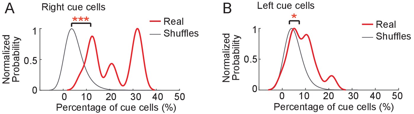
Comparison of the percentage of cue cells identified using original and randomized cue templates.
(A) Comparison of the percentage of right cue cells identified using the right cue template to cells identified using randomized versions of the original cue template. The red curve shows the distribution of the percentages of cue cells identified using the current cue template (12 FOVs from four mice). The gray curve shows the distribution of the percentages of cue cells identified using random cue templates. The curve represents data from all 12 FOVs with 200 random cue templates generated for each FOV. The distributions for real and shuffled templates were estimated using a kernel smoothing function with the same bandwidth of the smoothing window. The maximal distribution probabilities of all real and shuffled data were normalized to 1. p value: 4.45 × 10⁻⁹. (B) Similar to A but for left cue cells. p value: 0.0168.
Figure 5—figure supplement 4
Cue cell properties in layers 2 and 3 of the MEC across different environments.
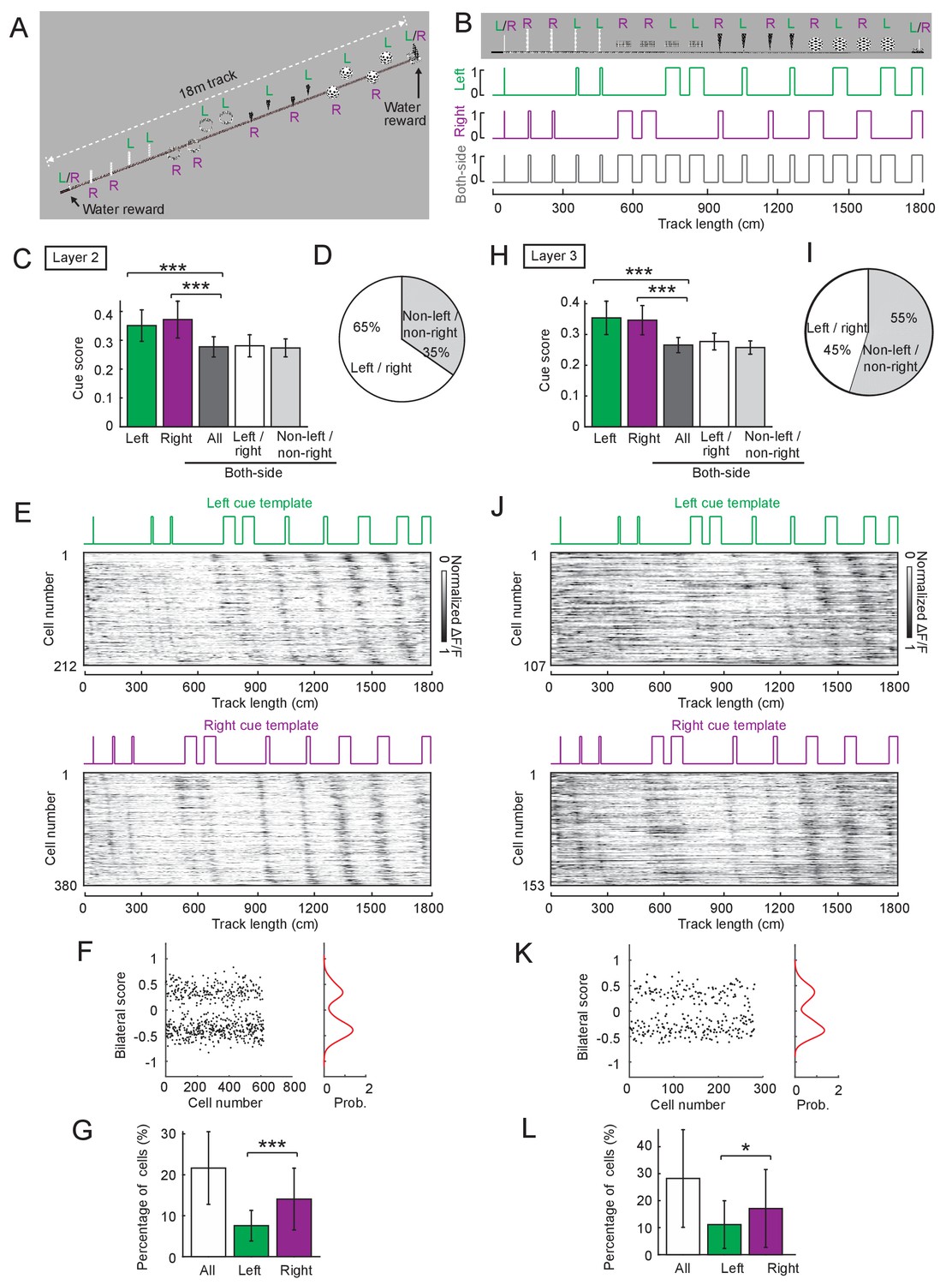
(A) An 1800 cm (18 meter) long virtual track for imaging experiments. ‘L’, ‘R’ and ‘L/R’ indicate cues on the left, right and both sides of the track, respectively. (B) Left, right, and both-side cue templates of the track in A. (C–G) Results for layer 2 cells, which were generated from 40 FOVs in six mice. (C) Comparison of cue scores. From left to right: scores of cells that passed the threshold of left, right, and both-side templates. Among the both-side cells, from left to right: all both-side cells; both-side cells that also passed thresholds of left and right templates; both-side cells that were not classified as left and right cells ( cells). Statistics: column 1 to 3: p=6.33 × 10−39, Column 2 to 3: p=6.90 × 10−52. (D) Pie chart showing the percentage of both-side cells that were also classified as left and right cells (white) and non-left and non-right cells (gray). (E) Cue cell sequences aligned to left- and right-side cues. Each row shows the mean ΔF/F along the track of a single cell, normalized by its maximum. The cells are sorted by the spatial shifts calculated from the correlation of the mean ΔF/F to the cue template. (F) Bilateral scores of left and right cells shown in C. Left: bilateral scores of individual cells (dots). Right: kernel density distribution of bilateral scores. Note that the distribution of bilateral scores is bimodal . (G) Percentages of cue cells. Left bar: all left and right cue cells. Middle bar: left cue cells. Right bar: right cue cells. Individual data points that were pooled for summary plots are cue cells from 40 FOVs in layer 2, p=7.12 × 10⁻⁶. (H–L) Similar to C-G but for layer 3 cells, from 37 FOVs in two mice. (H) Statistics: column 1 to 3: p=4.54 × 10⁻²⁸. Column 2 to 3: p=5.30 × 10⁻³². (L) Percentages of cue cells. Individual data points that were pooled for summary plots are cue cells from 37 FOVs in layer 3, p=0.041. *p≤0.05. ***p≤0.001. Student’s t-test.
-
Figure 5—figure supplement 4—source data 1
Cue scores, bilateral scores and percentages of cue cells in layers 2 and 3 on a 18-meter virtual linear track.
- https://cdn.elifesciences.org/articles/43140/elife-43140-fig5-figsupp4-data1-v2.mat
Figure 5—figure supplement 5

Spatial shifts of cells with cue-correlated activity patterns.
Method: The goal of this analysis is to investigate whether cells with cue-correlated activity patterns show consistently shifted responses to individual cues. Since cue cells were largely chosen based on the correlation of their activity patterns to a specific cue template (Figure 1B), this procedure could artificially select cells with activity patterns consistently shifted from individual cues and thus having high correlations to the template (comparability, high cue scores). Consequently, when these selected cue cells were ordered based on their spatial shifts, their responses were very likely to form consistent sequences at individual cues (as in Figures 4A and 5D). To avoid this artifact, here we classified cells with cue-correlated activity using a different approach in order to investigate whether having responses with consistent spatial shifts to individual cues is a true feature of cue cells. This analysis was performed on data collected in layers 2 and 3 of the MEC when mice navigated along an 18-meter track (Figure 5—figure supplement 4A and B). The track contained a large number of cues (10 cues), which allowed a more precise classification of cells with cue-correlated activity even when choosing only half the number of cues (method described below). Each cue template was split into two half-templates (templates 1 and 2), each containing half of the cues of the original template. The cues on the two templates were non-overlapping. Cue wells were first classified using one of the half-templates (i.e., template 1). The spatial shifts found from the correlation to template 1 was compared to that found for the other half-template (template 2), which was not used to classify the cells. The hypothesis was that if the response of a cue cell was shifted by the same distance from each cue, then the spatial shifts would be similar between these two half-templates. An example with two half-templates is shown in A. R1 and R2 are two half-templates with cues on the right side of the track. We calculated the percentage of cells that maintained similar spatial shifts across the two half-templates (the difference of the spatial shifts on R1 and R2 is less than 25 cm). We found that a large fraction of cue cells (76.9% and 80.3% for cells identified on R1 and R2, respectively) had very similar shifts on the two half-templates. A similar example for left-side cues is shown in (B). To further confirm that this high percentage of cells with consistent spatial shifts to cues was not found only by using a particular set of half-templates, we repeated this analysis for cells in both layers 2 and 3 using multiple sets of half-templates comprised of various combinations of cues from the original templates. This more strict analysis of spatial shifts of cue cells data together indicate that cue cells respond to individual cues with consistent spatial shifts.
Figure details: (A) Spatial shifts of cue cells classified using two half-templates of the right cue template (R template). The R template was split into two half-templates: R1 and R2. Spatial shifts of cue cells classified using R1 and R2 are shown in a1 and a2, respectively. a1: From top to bottom: (1) Classification of cue cells (R1 cue cells) using R1 template. (2) Ordered R1 cell responses based on their spatial shifts to R1 (R1 shifts). (3) Ordered R1 cell responses based on their spatial shifts to R2 (R2 shifts). Note that the activity patterns in both (2) and (3) consistently shift from individual cues, indicating that R1 cue cells generally had similar spatial shifts on R1 and R2. (4) Difference in spatial shifts of R1 cells on R1 and R2. Each dot is one cell. The fraction of cue cells (76.9%) with very similar spatial shifts on R1 and R1 (less than 25 cm absolute shift differences, marked by red parenthesis) a2: similar to a1 but for cue cells (R2 cue cells) classified using R2 template. (B) Similar to A but for left cue template (L template). (C) Summary of the percentages of cells in layers 2 and 3 with very similar spatial shifts (less than 25 cm absolute shift differences) on multiple pairs of half-templates (5 and 2 pairs for layers 2 and 3, respectively) comprised of different combinations of cues on the left and right cue templates (L1, L2, R1, R2). All analyses showed similar results. Red lines indicate the mean of each group.
Figure 6
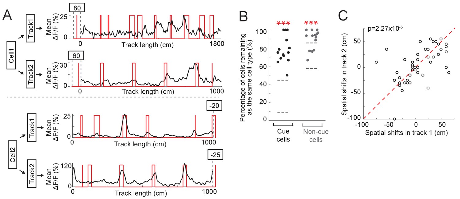
Cue cells respond to cues in different environments.
(A) Examples of two cue cells. Each cell was imaged on two tracks. For each cell: black: mean ΔF/F versus linear track position. Red: cue template. The spatial shift is shown above each plot (right and left shifts of the template relative to the mean ΔF/F curve are defined as negative and positive values, respectively). (B) Percentage of cue cells (black) and non-cue cells (gray) that remained as the same cell types in two tracks. Each dot represents one FOV (N = 14 FOVs in 5 mice, which formed 7 groups (two FOVs/group) to determine common cue cells for two tracks). For each cell type, the area between two gray lines represents mean ± STD of data on 50 random datasets, in which cue cells in two tracks were randomly assigned. Real data vs. random data: cue cell: p=1.46 × 10⁻²⁴; non-cue cell: p=5.13 × 10⁻¹⁴. (C) Spatial shifts of the same cue cells on two tracks. Each circles show the shifts of one cell. As in A, right and left shifts of the template relative to the mean ΔF/F curve are defined as negative and positive values, respectively. ectively. Red dotted line represents x = y. p=2.27 × 10⁻⁵. ***p≤0.001. Student’s t-test.
-
Figure 6—source data 1
Percentages of common cue and non-cue cells, and spatial shifts of common cue cells in different environments.
- https://cdn.elifesciences.org/articles/43140/elife-43140-fig6-data1-v2.mat
Author response image 1
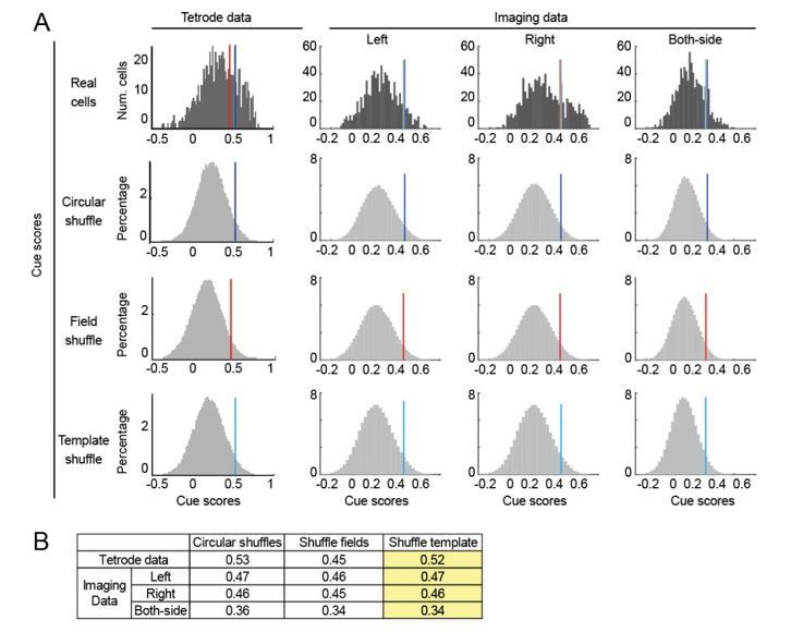
Score thresholds calculated by different shuffling methods.
(A) The distribution of shuffled cue scores and thresholds using three shuffling methods: circular permutation (circular shuffle), spatial field shuffle (field shuffle), and cue template shuffle (template shuffle). The thresholds values (95th percentile of shuffles) are indicated by dark blue, red and light blue lines, respectively. Left: distribution of real and shuffled cue scores for tetrode and imaging data. Right: distribution of real and shuffled cue scores for imaging data. Thresholds for left, right and both-side templates were separately calculated. B) Comparison of the thresholds generated by all three shuffling methods for tetrode and imaging data. In the current manuscript, we used the template shuffling method (highlighted in yellow).
Author response image 2
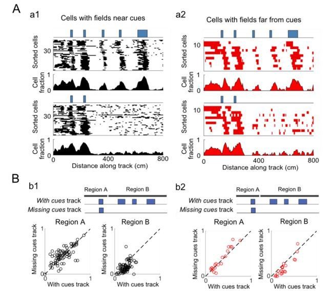
Cue-removal responses of cue cells with fields near or far from cues.
(A) Cue cells were sorted into two groups based on the spatial shift of their spatial firing rate relative to the cue template. Cells with spatial shifts less and more than 25 cm in either direction were categorized as cells with fields near and far from cues, respectively. a1: Top: spatial firing fields of all cue cells with fields near cues and the fraction of cells within each 5 cm bin with firing fields. Bottom: spatial firing fields and distribution of firing fields for the population of cells with fields near cues is shown for the track with the cues missing along the latter part of the track. a2: Similar to the plots in a1 but for cells with spatial firing fields far from cues. B) Summary plots: the fraction of bins with fields (field bins) for each cell is plotted for cells with fields near and far from cues on different track regions. b1: summary plots for cells with fields near cues. Left: the fraction of field bins for each cell in the early region of the track in which cues are present for both the “With cues” and “Missing cues” tracks (Region A). Right: the same type of plot for the latter part of the track where cues are present on the “With cues” track and missing on the “Missing cues” track. b2: summary plots for cells with fields far from cues. The dotted lines are drawn diagonally (slope=1).
Author response image 3
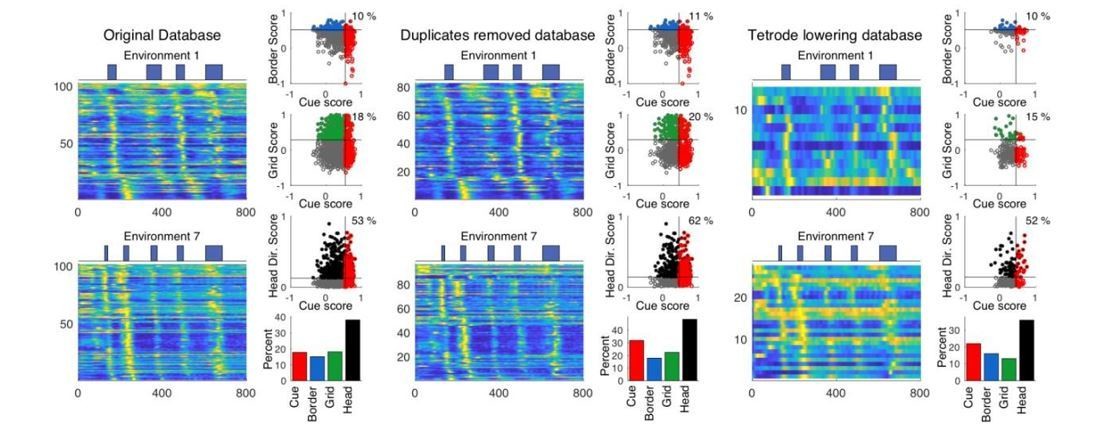
Trimming the tetrode database.
Cue cell sequences and scores for three different subsets of the tetrode database. Left: the original database from the original manuscript is shown. Middle: the new trimmed database with duplicates across days removed. Right: database in which cells recorded on the days in which a given tetrode was lowered are kept. In each of the three panels, the sequences of cue cells found in the database for environments 1 and 7 are shown on the left. To the right, the cue scores versus border, grid, and head direction score are shown, as well as the overall distribution of cell types.
Author response image 4
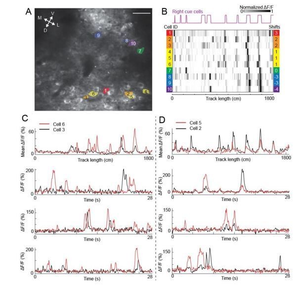
Calcium transients of anatomically adjacent cells with similar spatial shifts.
A and B are figure panels in the previous Figure 7G and H. C) Calcium responses of cell 3 (black) and cell 6 (red). Top: mean ΔF/F. Second to bottom: three examples of calcium traces (ΔF/F) showing that the shapes of calcium transients (large peaks) and the patterns of baseline activity of the two cells are different. D) Similar to C but for cell 5 and cell 2.
Tables
Key resources table
| Reagent type (species) or resource | Designation | Source or reference | Identifiers | Additional information |
|---|---|---|---|---|
| Strain, strain background (Adenovirus) | AAV1.hSyn.GCaMP6f.WPRE.SV40 | Penn Vector Core/addgene | Cat#: 100837-AAV1 | |
| Genetic reagent (M. musculus) | C57BL/6J | Jackson Laboratory | Stock No: 000664|Black 6 | |
| Genetic reagent (M. musculus) | Thy1-GCaMP6f transgenic line (GP5.3) | Janelia Research Campus; PMID:25250714 | N/A | Male and female |
| Commercial assay | NeuroTrace | Thermo Fisher Scientific | Cat#: N21479 | |
| Software, algorithm | MATLAB | MathWorks | https://www.mathworks.com | |
| Software, algorithm | ImageJ | National Institutes of Health | https://imagej.nih.gov/ij/ | |
| Software, algorithm | ScanImage 5 | Vidrio Technologies | http://scanimage.vidriotechnologies.com/display/SI5/ScanImage+5 | |
| Software, algorithm | ViRMEn (Virtual Reality Mouse Engine) | PMID:25374363 | https://pni.princeton.edu/pni-software-tools/virmen | |
| Software, algorithm | Motion correction (CaImAn) | PMID:30652683 | https://github.com/flatironinstitute/CaImAn |
Additional files
Download links
A two-part list of links to download the article, or parts of the article, in various formats.
Downloads (link to download the article as PDF)
Open citations (links to open the citations from this article in various online reference manager services)
Cite this article (links to download the citations from this article in formats compatible with various reference manager tools)
Visual cue-related activity of cells in the medial entorhinal cortex during navigation in virtual reality
eLife 9:e43140.
https://doi.org/10.7554/eLife.43140


