Figures and data in Somatosensory neurons integrate the geometry of skin deformation and mechanotransduction channels to shape touch sensing | eLife

Figures
Additional files

21 figures and 2 additional files

Figures

Figure 1

Download asset Open asset

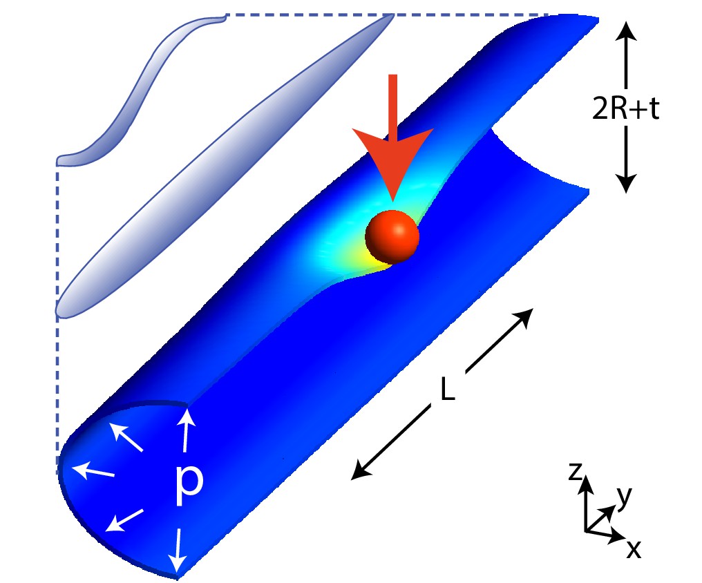
Scheme of the geometry in our model for C. elegans mechanics.

The figure shows the scheme of a worm in a natural posture (left), straightened (as in neurophysiology experiments), and the model (right) that we shall consider here: a cylinder of length $L ≃ 1 m m$ and radius $R + t / 2 ≃ 25 μ m$ is indented by a spherical bead (with radius 10 μm unless stated otherwise), applied here at its center. $R$ is the radius of the middle surface and $t$ is the thickness of the shell. Only half of the cylinder is shown for clarity.

https://doi.org/10.7554/eLife.43226.002

Figure 2

Download asset Open asset

Deformation profiles and force indentation relations.

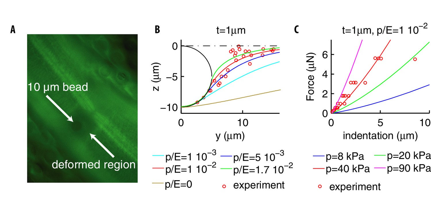
(A) Representative photomicrograph of a transgenic animal with GFP-tagged cuticular annuli being pressed into a glass bead. Experimental deformation profiles in (B) were derived from a stack of images at different focal planes. (B) Experimental and numerical deformation profiles along the longitudinal axis (the generatrix of the cylinder). Data were obtained as described in Materials and methods by using 2 biological replicates (adult animals). (C) Experimental (from Eastwood et al., 2015; Eastwood et al., 2019) and numerical force-indentation relationships. Length is $L = 1 m m$ and the Poisson coefficient $ν = 0.3$ .

https://doi.org/10.7554/eLife.43226.003

Figure 2—source data 1 Measurements of cuticle deformation by beads.: https://doi.org/10.7554/eLife.43226.004
Download elife-43226-fig2-data1-v1.xls

Figure 3

Download asset Open asset

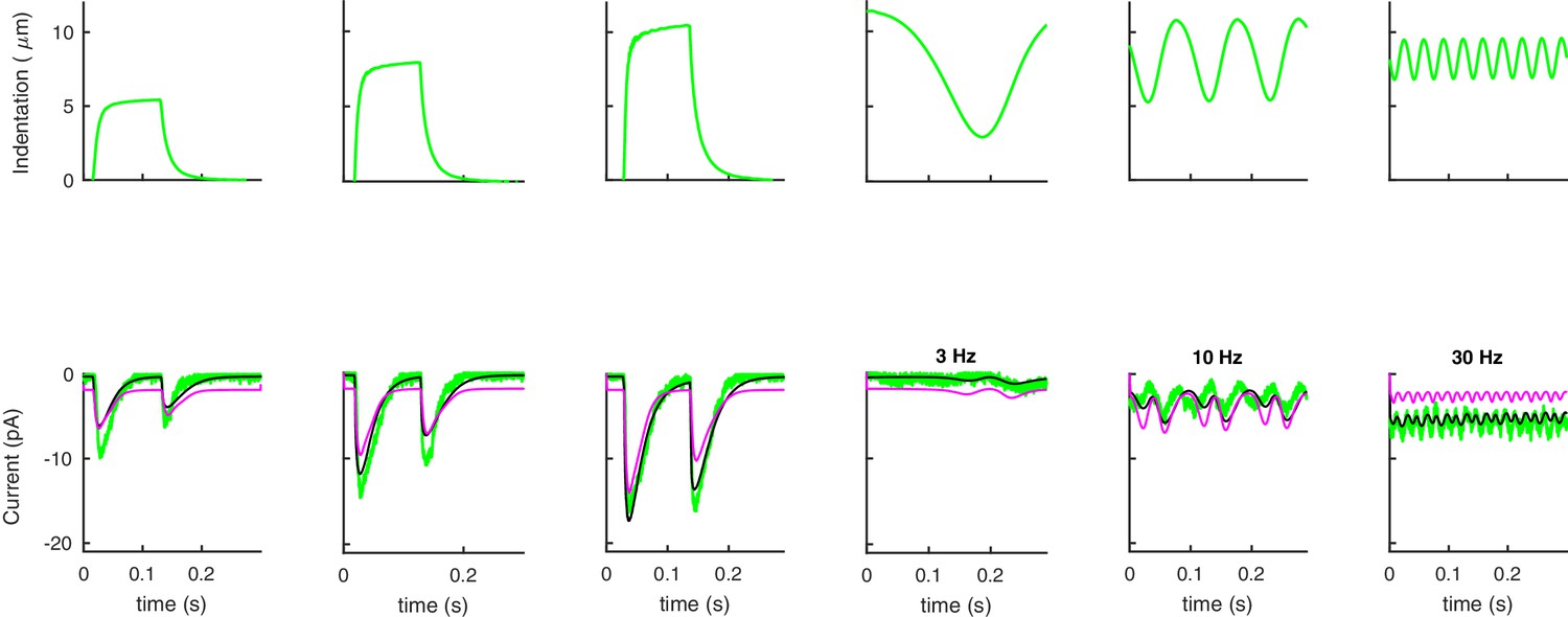
Our model captures experimental neural responses to various stimuli.

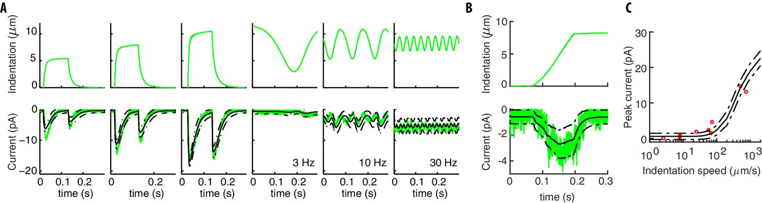
(A) The applied experimental indentation (top); TRN’s response (bottom, green) and average predictions (solid black). Dot-dashed black lines correspond to one standard deviation above/below the mean. Experimental stimuli and neural responses are from Eastwood et al. (2015) and Eastwood et al. (2019). (B) A typical ramp-like profile of indentation (top) and the corresponding current (TRN’s response in green; black lines as in panel A). (C) The predicted peak current vs the slope of the ramp for a total fixed indentation of 8 μm. Red circles indicate experimental data from Eastwood et al. (2015) and Eastwood et al. (2019).

https://doi.org/10.7554/eLife.43226.005

Figure 4

Download asset Open asset

Pre-indented steps yield stronger responses due to their more extended deformation profile.

(A) Stimuli delivered for standard (blue) and pre-indented (purple) steps. Black arrows indicate the total displacements for the on-currents in the following panels (colors match). Green arrows indicate relative displacements. Experimental stimuli and neural responses from ALM neurons were obtained as detailed in Materials and methods. We recorded from 11 separate worms with 3 − 11 presentations of each stimulus per recording. Recordings were only included if they met the criteria outlined in the Data Analysis section of the experimental methods, which led to a final number of biological replicates per displacement point that varied from 5 to 11. Representative traces shown here are from one biological replicate. (B) The on-current vs the total displacement (the pre-indentation for the purple points is 5 μm). Dotted curves and diamonds (in this panel and the following ones) report the prediction of our previous Mean Field (MF) model in Eastwood et al. (2015). The goal is to stress the importance of spatial integration effects, which constitute the main contribution of this paper and were neglected in Eastwood et al. (2015). (C) Off-currents are statistically indistinguishable, as expected since off-steps are identical and adaptation erased the memory of the pre-step. (D) The on-current vs the relative displacements. Note the stronger response for pre-indented stimuli. (E) Changes in the profile of deformation: $Δ z$ is the difference between the deformations after and before the (relative) stimuli. Note the greater extension for the pre-indented case, which is the reason underlying results in panel D. Open circles in panels B-D were normalized to the maximal currents detected and show the mean ± s.e.m.

https://doi.org/10.7554/eLife.43226.006

Figure 4—source data 1 Experimental and simulated neural responses to pre-indented steps.: https://doi.org/10.7554/eLife.43226.007
Download elife-43226-fig4-data1-v1.xls

Figure 5

Download asset Open asset

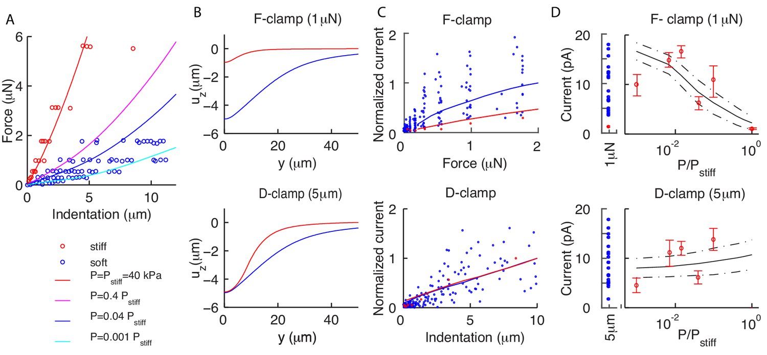
Residual internal pressure accounts for current amplitude in soft and stiff worms.

(A) Experimental data (dots) and the average theoretical prediction (lines) for force-indentation relations. Best fit of pooled data for soft worms gives $p$ = 1.6 kPa; individual values are variable, with estimated $p$ in the range 0.04–16kPa. (B) The vertical deformation profiles $u_{z}$ vs the position $y$ along the longitudinal axis for stiff (red) and soft (blue) animals. Note the widely differing profiles for the force-clamped curves. (C) Experimental (dots) and theoretical (mean value as continuous lines) peak current for force (top) and displacement-clamped (bottom) stimuli. The current is normalized by the mean peak in soft and stiff worms, respectively. (D) Peak current vs the pressure $p$ , which shows that the model (continuous lines are the mean; dot-dashed lines are above/below one standard deviation) captures experimental trends (dots). Experimental data reproduced from Eastwood et al. (2015) and Eastwood et al. (2019) and derived from 4 and 21 recordings in the stiff (red) and soft (blue) conditions, respectively.

https://doi.org/10.7554/eLife.43226.008

Figure 5—source data 1 Experimental and simulated neural responses to force-clamped or displacement-clamped stimuli.: https://doi.org/10.7554/eLife.43226.009
Download elife-43226-fig5-data1-v1.xls

Figure 6

Download asset Open asset

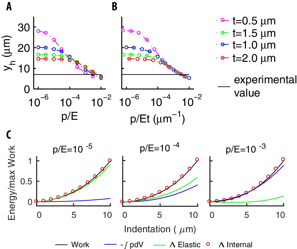
The mechanical balance for our model of pressurized shell.

(A) The longitudinal extension $y_{h}$ vs $p / E$ for various thicknesses $t$ . Different trends at small and large values of $p / E$ reflect the contributions of bending to the elastic energy. (B) $y_{h}$ vs $p / E t$ . The collapse of the curves at the right end reflects the small value of the bending term coefficient (see the text). The value of $y_{h}$ found experimentally (black line) is well inside that asymptotic region. (C) The various contributions to energy, and the work done by the indenter for increasing values of the ratio $p / E$ .

https://doi.org/10.7554/eLife.43226.010

Figure 7

Download asset Open asset

Effects of the radius $R_{b}$ of the indenting bead.

(A) In pressurized shells, the deformation profile depends on $R_{b}$ (colored lines) while the dependence disappears in the absence of internal pressure (black line). (B) The force-indentation relation for $p = 40 k P a$ and various $R_{b}$ . In strongly pressurized shells, the relation (colored dots) follows Equation (12) (solid lines). For shells with $p = 0$ , the curves collapse onto a unique curve (black dots). (C) The ratio $F (w_{0}) / F_{m a x}$ of the force normalized by its maximum value is essentially independent of $R_{b}$ . (D) The peak current increases with $R_{b}$ in a $p$ -dependent manner (the same holds for the sensitivity to the stimulus). The current is normalized by its value for $R_{b} = 5 μ m$ .

https://doi.org/10.7554/eLife.43226.011

Figure 8

Download asset Open asset

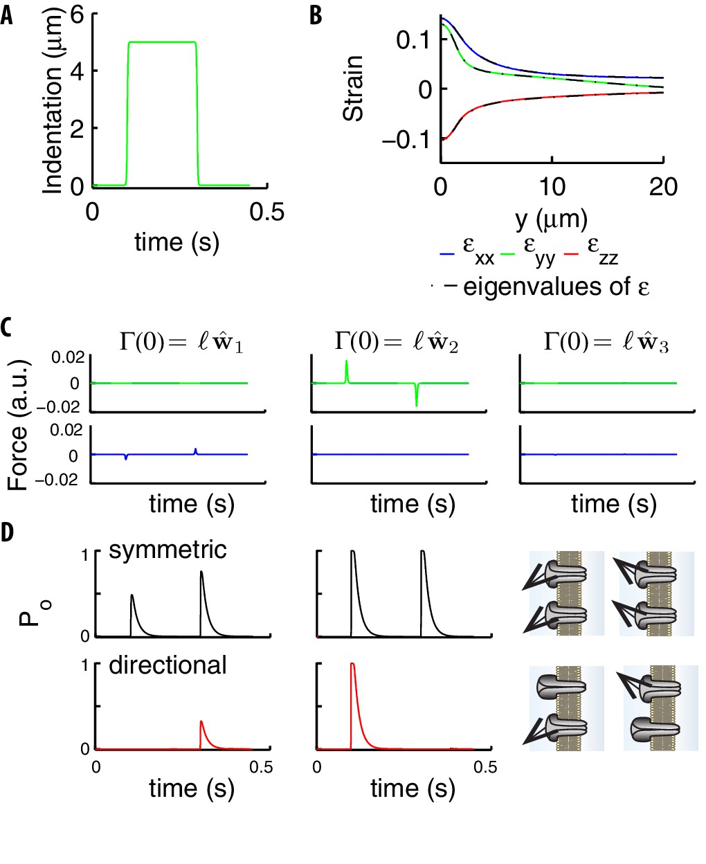
Stimuli on the channels due to a step.

(A) Indentation profile for a step stimulus. (B) The diagonal components of the strain tensor $ε_{i j}$ vs the longitudinal position along the cylinder. The overlap of those components (color) and the eigenvalues of $ε_{i j}$ (black) show that the tensor is essentially diagonal, which leads to the conservation of angles under deformation discussed in the main text. (C) The two components (green and blue curves) tangential to the neural membrane of the force acting upon on a channel (computed using Equations (5), (9)) for the stimulus in panel A. The panels refer to the different directions of the elastic filament (the first two are tangential and the third orthogonal to the neural membrane). (D) Gating probability for an individual symmetric or directional channel, as produced by the two tangential extensions in panel C. Parameters are: $y = 1 μ m$ , $θ = 0$ , $𝑣 = \cos (π / 3) {\hat{𝐰}}_{1} - \sin (π / 3) {\hat{𝐰}}_{2}$ . The sketch on the right illustrates that directional channels respond only to stimuli properly aligned with respect to their preferential direction while symmetric channels respond isotropically.

https://doi.org/10.7554/eLife.43226.012

Figure 9

Download asset Open asset

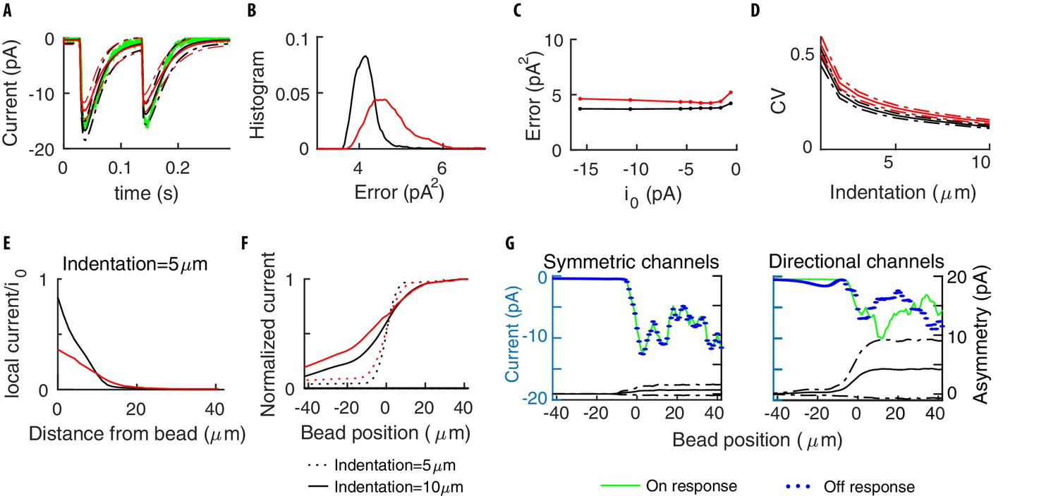
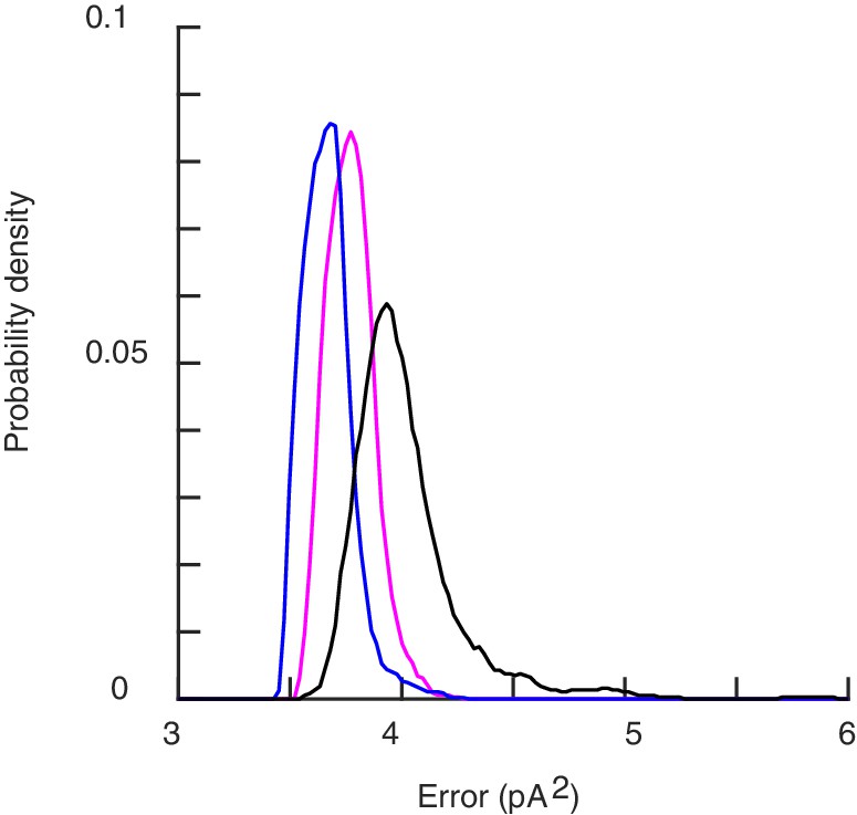
Symmetry of the single channel response.

(A) Mean neural current response to a step, for symmetric (black) vs directional (red) channels. (B) Histogram of the errors in reproducing the data of Figure 3 obtained with the two above models for different realizations of the channels’ distribution. Symmetric channels (black) give a better description. (C) The mean error as the maximum current $i_{0}$ per channel is varied. (D) The Coefficient of Variation (CV) of the TRN current vs the stimulus strength, calculated over many repetitions of a given stimulus. (E) The average current for a channel (normalized by its maximum value $i_{0}$ ) as a function of its distance to the center of the indenting bead. (F) The current flowing along the TRN vs the position of the indenting bead. The origin indicates the end of the TRN; negative coordinates correspond to the relatively insensitive zone in the middle of the body of the worm. (G) The colored curves show the predicted current for symmetric and directional channels, for a given distribution of the channels. The black curves show the expected level of asymmetry between onset and offset, as quantified by the standard deviation ${⟨ {(I_{o n} - I_{o f f})}^{2} ⟩}^{1 / 2}$ between the peak responses $I_{o n, o f f}$ at the onset/offset of the stimulus, averaged over the distributions of the channels. Dashed-dotted curves show the range of expected asymmetries in individual realizations.

https://doi.org/10.7554/eLife.43226.013

Appendix 1—figure 1

Download asset Open asset

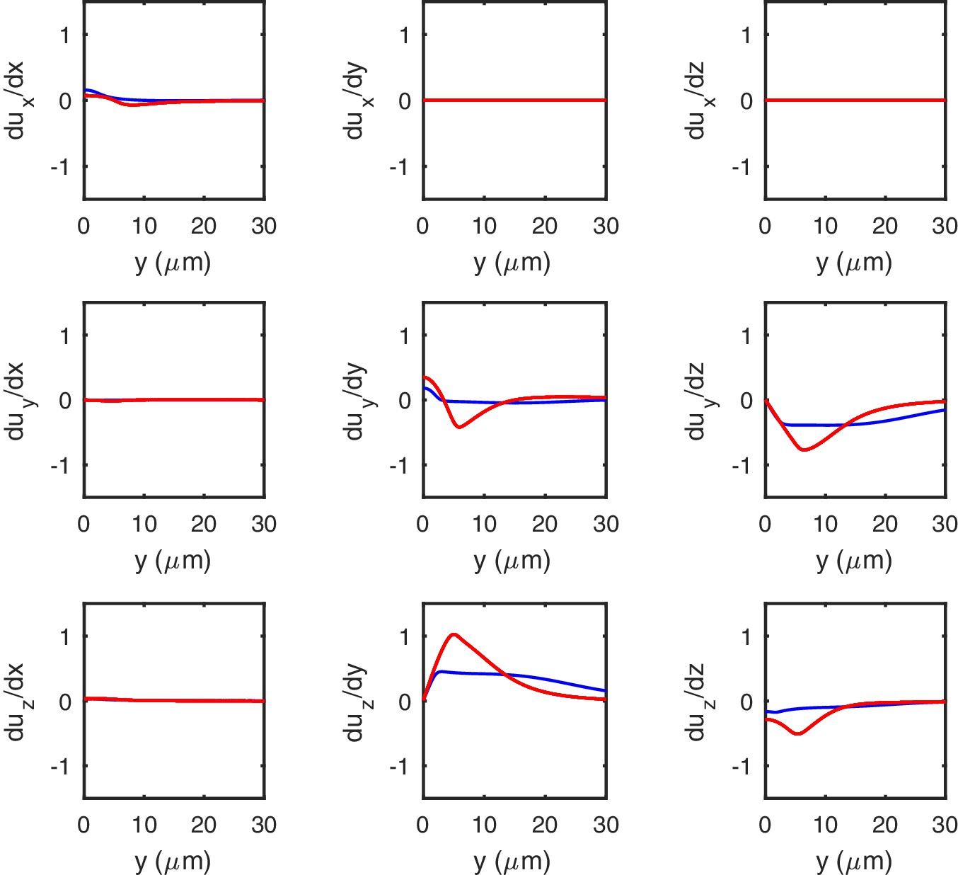
The gradients of the deformation along the longitudinal direction of an indented cylinder.

Gradients of $𝐮$ computed by using numerical simulations for soft ( $p / E = 4 \times 10^{- 4}$ , blue) and stiff ( $p / E = 0.01$ , red) shells. Note their moderate amplitude even for the indentation of 10 μm shown here, which is the strongest that we consider.

https://doi.org/10.7554/eLife.43226.017

Appendix 2—figure 1

Download asset Open asset

Deformations of a cylindrical shell due to internal pressure.

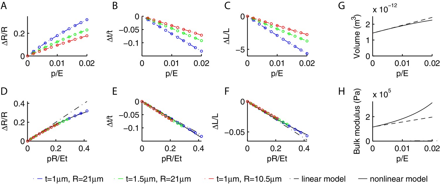
Relative change in the radius $R$ (A), thickness $t$ (B) and length $L$ (C) of the shell as a function of $p / E$ and various $t / R$ , as obtained from our numerical simulations. As $p$ increases, $R$ increases whilst $t$ and $L$ decrease. (D,E,F) While the curves in the previous panels change with $t / R$ , the curves are collapsed by plotting them against $p R / E t$ , which suggests that the contribution of terms in $t / R$ is negligible. The collapsed behavior agrees with the linear prediction Equation (21) for $p R / E t < 0.1$ (dash-dotted lines), and is well captured by the empirical Equation (23) in the moderately nonlinear regime. Using the nonlinear Equation (23), we computed the change in volume (G) and bulk modulus (H) of the shell as a function of $p / E$ (dashed lines are the linear predictions Equation (22) valid for small values of $p / E$ ).

https://doi.org/10.7554/eLife.43226.019

Appendix 3—figure 1

Download asset Open asset

Effect of atmospheric pressure on mechanical response.

Deformation profile (first row) and force indentation relation (second row) for a cylindrical shell (with the same properties as in the main text) with (purple) and without (black) atmospheric pressure.

https://doi.org/10.7554/eLife.43226.021

Appendix 3—figure 2

Download asset Open asset

Effect of atmospheric pressure on neural response.

Neural responses of the model presented in the main text to the experimental stimuli in Figure 3 of the main text. Green curves are experimental data (as in Figure 3 of the main text); purple and black curves are model predictions with and without atmospheric pressure, respectively. The ratio $p / E$ is 7‰ of the value for stiff worms.

https://doi.org/10.7554/eLife.43226.022

Appendix 5—figure 1

Download asset Open asset

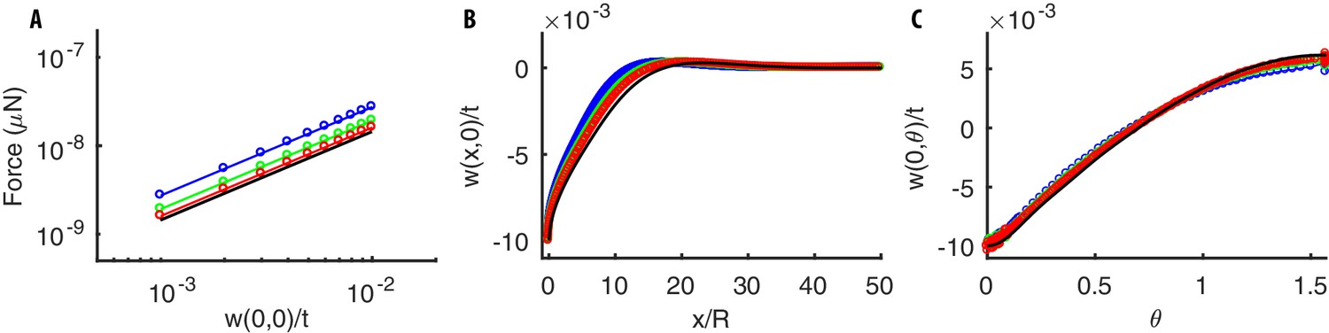
Mechanical response of a thin cylindrical shell to equal and opposite concentrated radial loads.

(A) Force-indentation relation. (B–C) Radial deflection along the longitudinal and angular directions. The analytical solution Equation (30) (black line) is well approximated by numerical solutions (colored lines) obtained by using our numerical code. The agreement improves as the numerical mesh becomes finer (the mesh length is $t$ (blue), $t / 2$ (green), $t / 3$ (red), where $t$ is the thickness of the shell). Parameters of the simulations are: $t / R = 10^{- 2}$ , $t = 1 μ$ m, $E = 1$ MPa, $ν = 0.3$ .

https://doi.org/10.7554/eLife.43226.025

Appendix 5—figure 2

Download asset Open asset

Mechanical response of a pressurized thin spherical shell to a point indentation at the north pole.

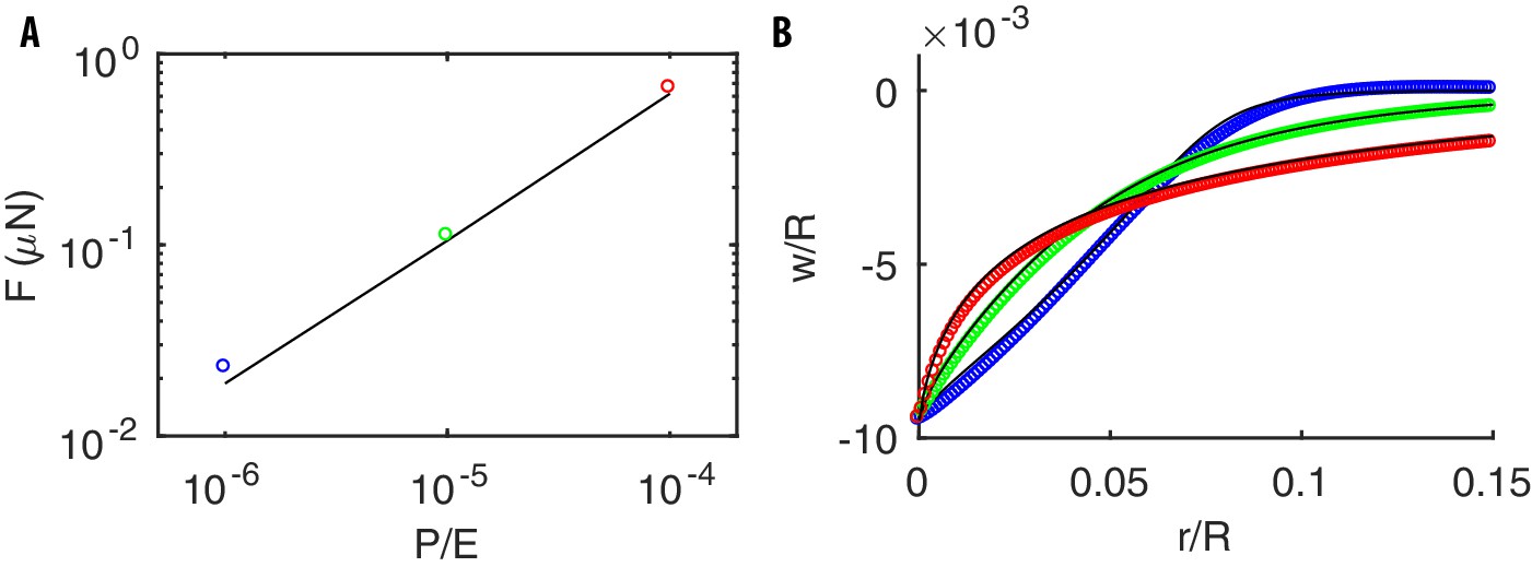
(A) The force required to produce a deformation $w_{0} / R = - 10^{- 2}$ for different values of $p$ . (B) The deformation profile for $p / E = 10^{- 6}$ (blue), $10^{- 5}$ (green), $10^{- 4}$ (red). Black lines and colored dots correspond to the solutions of Equation (32) and the results by our code, respectively. Note that, as for a pressurized cylinder (see main text), the deformation profile narrows as $p$ increases. Parameters of the simulations are : $E = 1$ MPa, $ν = 0.3$ , $t / R = 10^{- 3}$ , $t = 1 μ$ m.

https://doi.org/10.7554/eLife.43226.026

Appendix 6—figure 1

Download asset Open asset

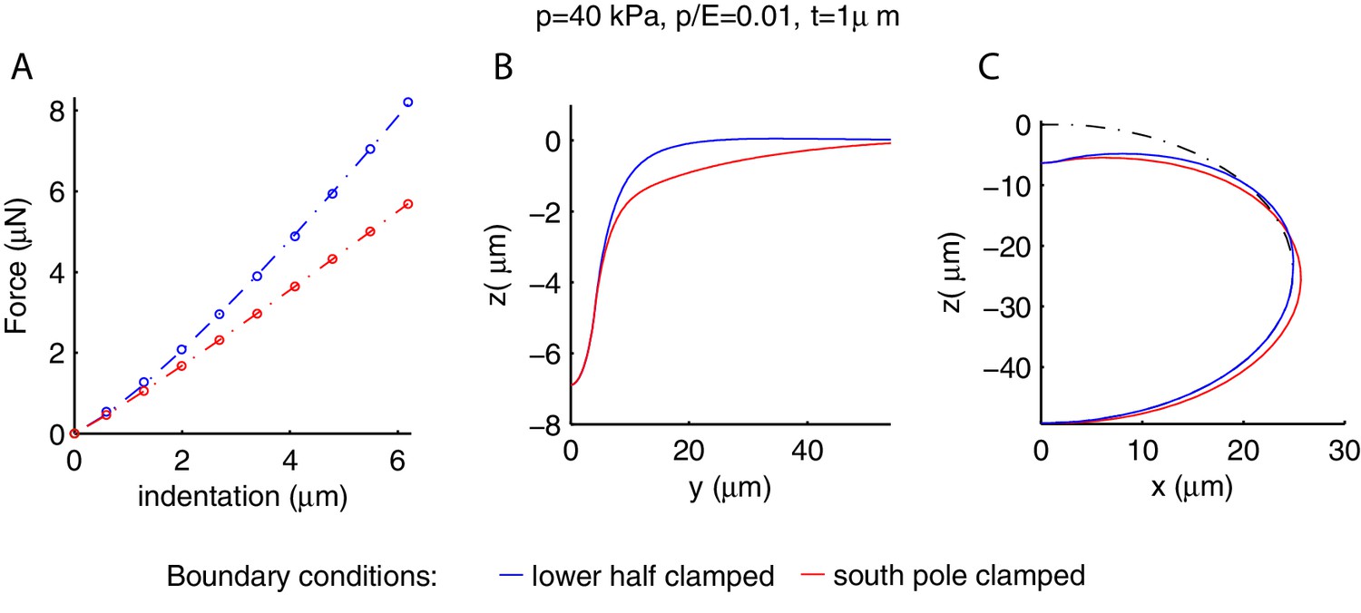
Influence of the gluing of the worm on its mechanical response.

Blue and red curves correspond respectively to gluing of the entire lower half of the cylinder or the line of contact with the plate (south pole) only. (A) Force-indentation relations; note that the stiffness is greater for the blue curve. The deformation profiles along the longitudinal (B) and orthogonal (C) directions are wider for the south-pole gluing, which has the lower half of the shell deformed in the orthogonal direction as well. The undeformed geometry is the black dash-dotted line.

https://doi.org/10.7554/eLife.43226.028

Appendix 7—figure 1

Download asset Open asset

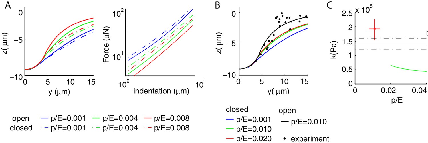
Boundary conditions at the ends of the shell influence mechanical properties.

(A) Comparison of the mechanical response for a closed (dash-dot line) and open (continuous line) cylinder. For a given value of $p / E$ , the deformation profile is more extended (left) and the shell stiffer (right) if the two ends are closed; the difference increases with $p / E$ . (B) Experimental and numerical deformation profiles along the longitudinal axis. None of the values $p / E \in [0, 0.02]$ for the closed cylinder (colored line) captures experimental data. (C) Experimental and predicted values for the bulk modulus. The value predicted for closed conditions at the ends decreases with $p / E$ and is too small to account for the data. Results for free lateral conditions are shown for comparison. Parameters of the simulations are as in Figure 2 of the main text.

https://doi.org/10.7554/eLife.43226.030

Appendix 9—figure 1

Download asset Open asset

The linear form of Equation (35) outperforms its quadratic counterpart in describing experimental data.

(A) The average predictions for the experimental data (green) given by the linear (black) and quadratic (purple) forms of Equation (35).

https://doi.org/10.7554/eLife.43226.033

Appendix 11—figure 1

Download asset Open asset

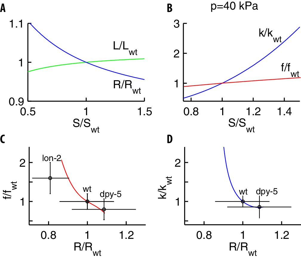
Changes in the mechanics caused by mutations of proteins in the cuticle.

Mutations are modeled via changes of the stretching stiffness $S$ with respect to the wild type $S_{w t}$ . (A) As $S$ increases, the geometry of the pressurized cylinder modifies: its length $L$ increases and its radius $R$ decreases. (B) As $S$ increases, the bulk modulus $k$ (blue) and the stiffness $f$ (red) of the force-indentation relation increase. (C–D) Our theoretical predictions and experimental measurements (Park et al., 2007; Gilpin et al., 2015) for $f$ and $k$ vs $R$ . Since the radius of the mutants was not reported in Gilpin et al. (2015), we used values in Park et al. (2007). The upshot is that lon-2 mutants should have a bulk modulus significantly different than the wild type.

https://doi.org/10.7554/eLife.43226.036

Appendix 13—figure 1

Download asset Open asset

Dependence of the neural response on the filament-medium interaction.

Peak current (A) and decay time (B) as a function of the relaxation time $τ$ of the elastic filament connected to the channel. The model predicts that both the peak current and the decay time increase with $τ$ .

https://doi.org/10.7554/eLife.43226.039

Appendix 13—figure 2

Download asset Open asset

Dependence of the neural response on the geometry of the filaments.

The error for the profiles of stimulation in Figure 3 of the main text. The black histogram is built from individual realizations for the unconstrained model discussed in the main text. The purple and the blue curves refer to the corresponding histograms for filaments initially or permanently restricted to be tangential to the neural membrane.

https://doi.org/10.7554/eLife.43226.040

Additional files

Supplementary file 1 Key Resources Table.: https://doi.org/10.7554/eLife.43226.014
Download elife-43226-supp1-v1.xlsx
Transparent reporting form: https://doi.org/10.7554/eLife.43226.015
Download elife-43226-transrepform-v1.docx

Download links

A two-part list of links to download the article, or parts of the article, in various formats.

Downloads (link to download the article as PDF)

Article PDF

Open citations (links to open the citations from this article in various online reference manager services)

Mendeley

Cite this article (links to download the citations from this article in formats compatible with various reference manager tools)

Alessandro Sanzeni
Samata Katta
Bryan Petzold
Beth L Pruitt
Miriam B Goodman
Massimo Vergassola

(2019)

Somatosensory neurons integrate the geometry of skin deformation and mechanotransduction channels to shape touch sensing

eLife 8:e43226.

https://doi.org/10.7554/eLife.43226

Sign up for email alerts

Privacy notice