Shared behavioral mechanisms underlie C. elegans aggregation and swarming
Figures
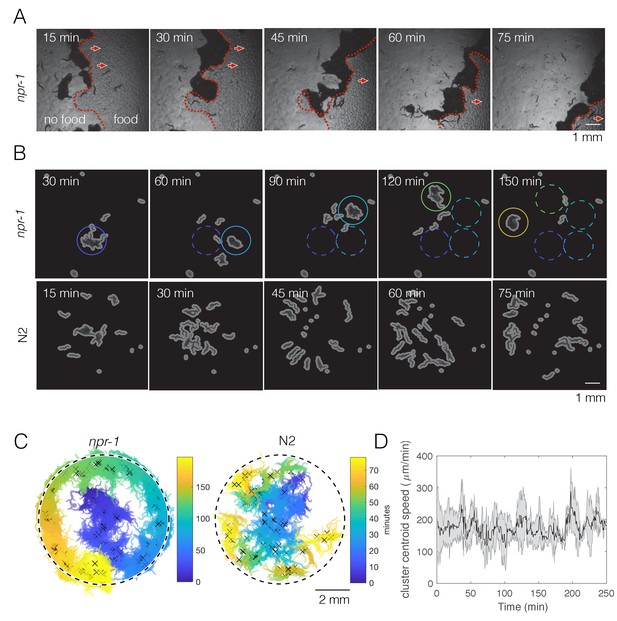
npr-1 but not N2 worms show swarming behavior over time on thin bacterial lawn.
(A) A few hundred npr-1 mutant worms form dense clusters that move on food over time. Red dashed lines show the food boundary, where area with food is to the right and food-depleted area is to the left; red arrows show the direction of cluster movement. (B) Forty npr-1 mutant worms also cluster and swarm on food. Solid circles encompass the same cluster at different time points; dashed circles show cluster positions prior to the current time point. The same number of N2 worms do not swarm under our experimental conditions, and instead disperse after initial transient aggregation. (C) Visualization of persistent swarming over time. One frame was sampled every 30 s over the duration of the videos and binary segmentation was applied using an intensity threshold to separate worm pixels from the background. Blobs with areas above a threshold value were plotted as clusters to show cluster position over time. The same videos as in (B) were used. Dashed circles show the food boundary. Crosses are cluster centroids at each sample frame. (D) Centroid speed of persistent npr-1 clusters, calculated from centroid positions as indicated in (C) and smoothed over 10 min. Shaded area shows standard deviation across five replicates.
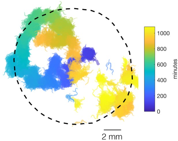
npr-1 swarming on a bigger food patch.
Forty npr-1 animals swarm over a big food patch, reminiscent of a persistent random walk. More than one large moving clusters co-exist towards the end of the video (orange and yellow), and a cluster (orange) disperses and re-forms elsewhere (orange and yellow) when it crosses its previous path (blue), presumably due to local food depletion.
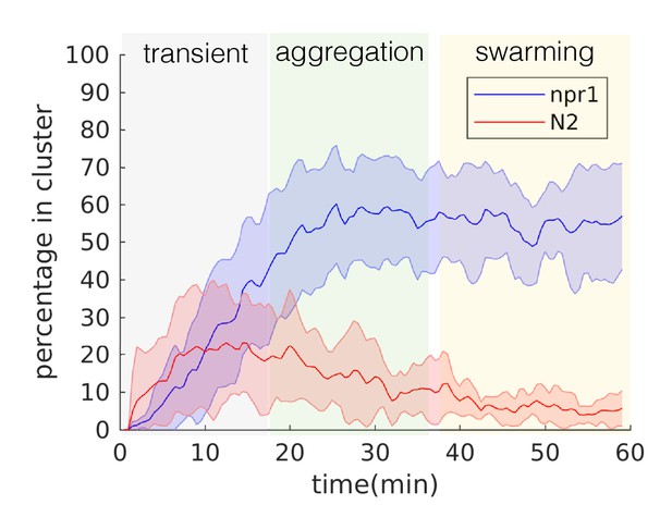
Stereotyped temporal dynamics.
One-hour fluorescence recordings of npr-1 animals under our experimental conditions consist of reproducible temporal dynamics encompassing three phases: transient (animals move about the lawn and start to form clusters), aggregation (clusters largely remain stable with individuals entering and exiting), and swarming (worms move across the lawn in persistent clusters) (see sample Video 2). Percentage of in-cluster worms remain largely consistent throughout the latter two phases, except that clusters remain in place during the aggregation phase and become dynamic during the swarming phase. Error bars represent standard deviation across 13 (npr-1) and 9 (N2) replicates. The average duration of each phase derived from npr-1 experiments are applied to N2 data to maintain temporal consistency, even though N2 does not exhibit aggregation or swarming. Subsequent quantitative analyses for both strains were restricted to using the data from the aggregation (for all but Figure 1D) or swarming (for Figure 1D) phase, in order to reveal the mechanisms necessary for producing aggregation or the dynamics of swarming, respectively.
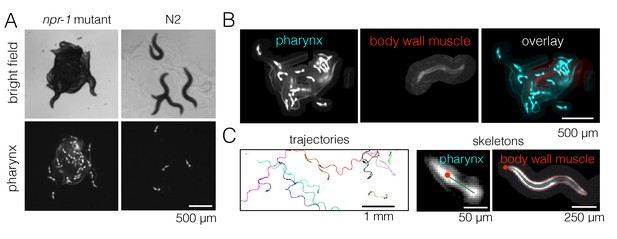
Fluorescence multi-worm tracking.
(A) npr-1 mutant and N2 animals exhibit different social behaviors on food, with the former being hyper-social (top left) and the latter being hypo-social (top right). Using a pharynx-GFP label (bottom row), individual animals may be followed inside a cluster. (B) In two-color experiments, worms are either labeled with pharynx-GFP (left) or body wall muscle-RFP (middle). As the two colors are simultaneously acquired on separate channels, the selected few RFP-labeled individuals are readily segmented and may be tracked for a long time, even inside a dense cluster. (C) Tierpsy Tracker tracks multiple worms simultaneously, generating both centroid trajectories (left, image color inverted for easier visualization; multiple colors show distinct trajectories) and skeletons (middle, pharynx-marked animal; right, body wall muscle-marked animal; red dots denote the head nodes of the skeleton).
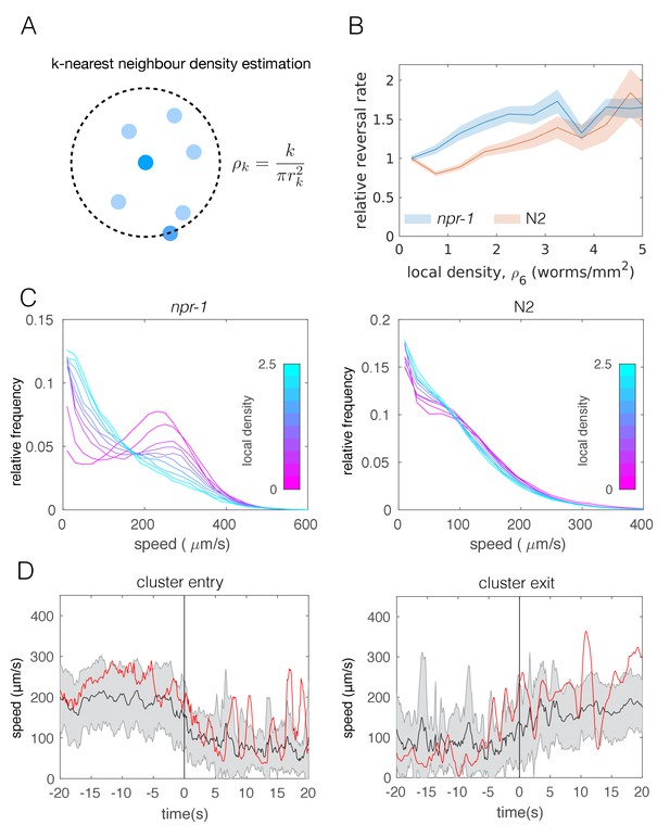
Individual-level behavioral quantification.
(A) Schematic explaining k-nearest neighbor density estimation. (B) Relative rate of reversals as a function of local density (k-nearest neighbor density estimation with k = 6) for npr-1 (blue) and N2 (orange) strains. Lines show means and shaded area shows the standard error (bootstrap estimate, 100 samples with replacement). (C) Distributions of crawling speeds at different local neighbor densities for both strains. Lines show histograms of speeds for each density bin, and the color of the line indicates the density (blue is high, magenta is low). (D) Midbody absolute speed for manually annotated npr-1 cluster entry (left, n = 28) and exit events (right, n = 29). Each event was manually identified, with time 0 representing the point where the head or tail of a worm starts to enter (left) or exit (right) an existing cluster. Skeleton xy-coordinates were linearly interpolated for missing frames for each event, before being used to calculate midbody speed extending 20 s on both sides of time 0 of the event. Speeds were smoothed over a one-second window. Shading represents standard deviation across events. Each red line shows the midbody absolute speed of a selected event that is shown in Video 3 (left) or Video 4 (right).
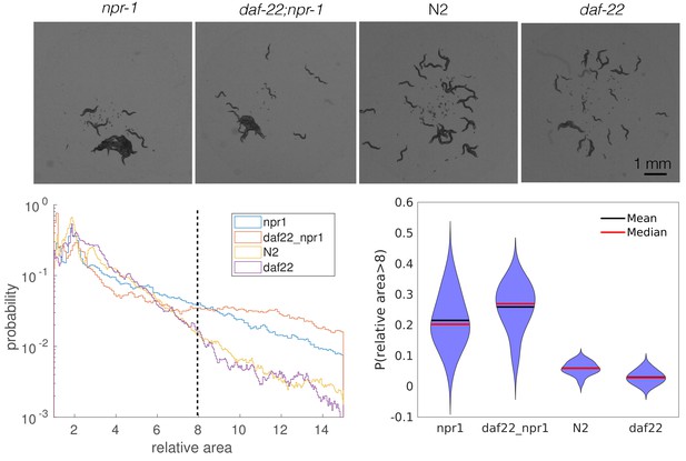
Pheromones appear unimportant for aggregation.
npr-1 and N2 animals with pheromones removed by a daf-22 mutation aggregate to similar levels as their pheromone-intact counterparts. Top row: snapshots of 40 worms from each strain behaving on a thin, uniform lawn. Bottom left: quantification of cluster area relative to single worm area for each strain; dashed line shows the cut-off values used to generate the violin plot on the bottom right. Bottom right: probability of having a relative cluster area above the threshold value (dashed line on the bottom left). Blob area were extracted as tracking features. For each recording, a random sample (without replacement) of 500 single worms was used to calculate single-worm mean area, which was used to normalize multi-worm cluster areas from that recording. Relative cluster area values for each strain were pooled across recording replicates, and histograms were created with a bin width of 0.5.
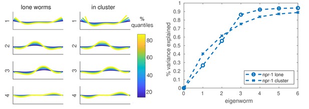
Shape analysis for lone and in-cluster npr-1 worms.
Left two panels: first four eigenworms (Stephens et al., 2008) plotted in real space for projections of lone worms and in-cluster worms. Right: variance explained as a function of the number of eigenworms. Eigenworms are based on common reference (Brown et al., 2013) set for both strains and worm categories.
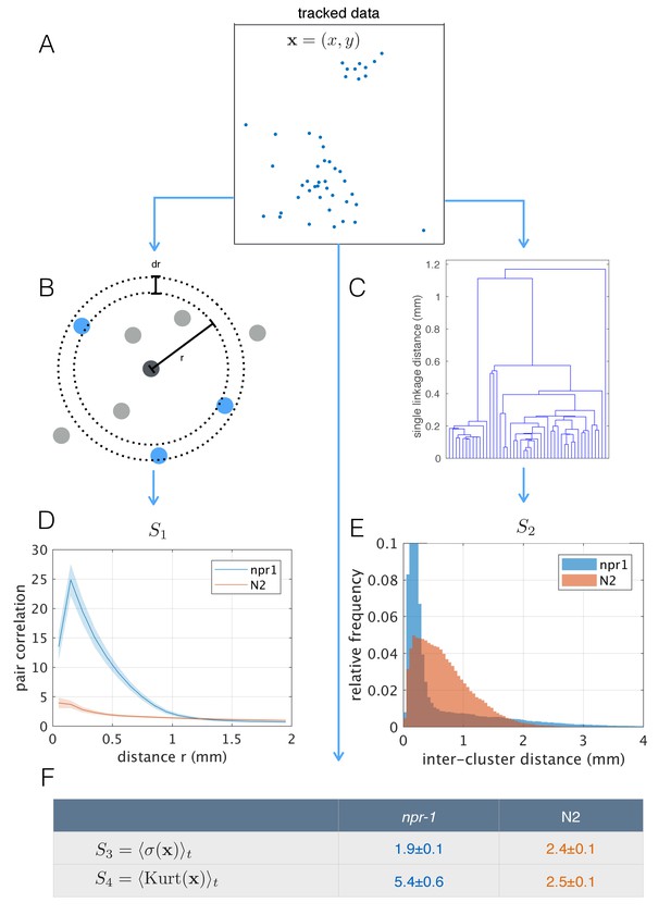
Population-level behavioral quantification.
(A) Positions of npr-1 worms in an example frame. (B) Schematic explaining pair correlation function (S1), which counts the number of neighbors at a distance r, normalized by the expectation for a uniform distribution. (C) Example dendrogram from which hierarchical clustering branch length distributions (S2) can be calculated. (D) Pair correlation function for npr-1 (blue) and N2 (orange). Lines show mean and shaded area shows standard error of the mean. (E) Hierarchical clustering branch length distributions for npr-1 (blue) and N2 (orange). Histograms show relative frequency of inter-cluster distances (single linkage distance in agglomerative hierarchical clustering, equivalent to the branch lengths in the example dendrogram in (C)). (F) Mean standard deviation (S3) and kurtosis (S4) of the positions of worms, with the mean taken over frames sampled.
Agent-based modeling of emergent behavior.
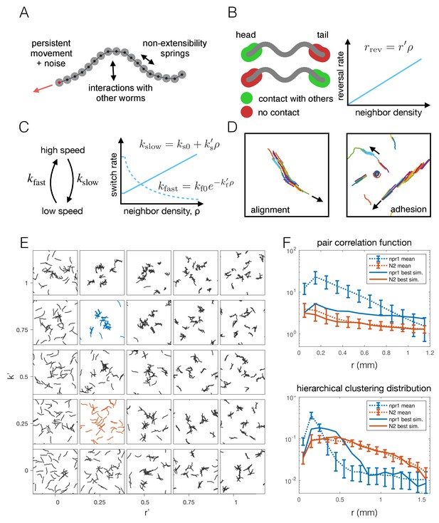
(A) Schematic of individual worm in the agent-based model. Each worm is made up of M nodes (here M = 18), connected by springs to enforce non-extensibility. Each node undergoes self-propelled movement, with the head node (red dot) undergoing a persistent random walk, and the rest of the nodes follow in the direction of the body. (B) Schematic of simulated reversals upon exiting a cluster. Each worm registers contact at the first and last 10% of its nodes within a short interaction radius. If contact is registered at one end but not the other, the worm is leaving a cluster and thus reverses with a Poisson rate dependent on the local density. (C) Schematic of density-dependent switching between movement speeds. Worms stochastically switch between slow and fast movement with Poisson rates kslow and kfast, which increase linearly and decrease exponentially with neighbor density, respectively. (D) Snapshots of simulations with commonly considered aggregation mechanisms, which produce unrealistic behavior for worm simulations, with flocking and highly aligned clustering. Arrows indicate the direction of movement of large clusters. (E) Phase portrait of model simulations, showing snapshots from the last 10% of each simulation, for different values of the two free parameters: density-dependence of the reversal rate and density-dependence of speed-switching (here kslow = kfast). Blue and orange panels highlight best fit for npr-1 and N2 data, respectively. (F) Summary statistics S1 (pair correlation, top) and S2 (hierarchical clustering, bottom) for the simulation which most closely matches the experimental data for the npr-1 and N2 strains (blue and orange panels in (E), respectively).
Model with taxis captures quantitative aggregation phenotypes.
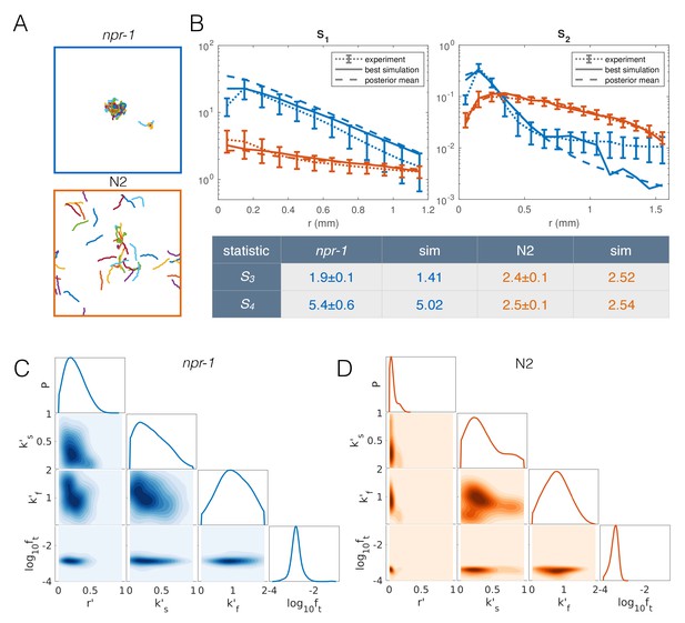
(A) Sample snapshot of the closest matching simulations for npr-1 (top) and N2 (bottom). (B) Summary statistics for npr-1 (orange) and N2 (blue): S1: pair correlation function; S2: hierarchical clustering distribution; S3: standard deviation of positions; S4: kurtosis of positions. Solid lines show the closest matching simulations; dashed lines show sample mean over the posterior distribution; and dotted lines show experimental means, with error bars showing standard deviation of 13 (npr-1) and 9 (N2) replicates. (C–D) Approximate posterior distribution of parameters for npr-1 (C) and N2 (D). Diagonal plots show marginal distribution of each parameter, off-diagonals show pairwise joint distributions. Parameters are: increase in reversal rate with density, r'; increase in rate to slow down, k's; decrease in rate to speed up, k'f; and contribution of taxis to motile force, ft.
Reduced prior distribution used for approximate Bayesian inference of extended model.
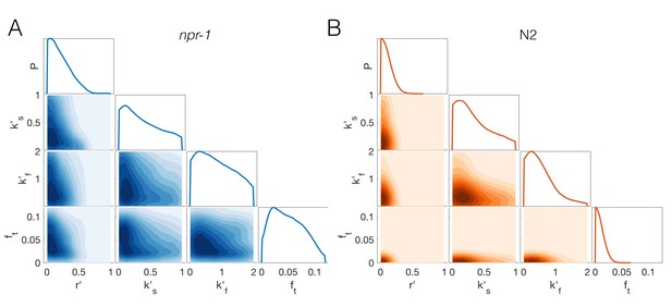
Marginal and joint prior parameter distributions for npr-1 (A) and N2 (B), that have been constructed from a set of pilot runs excluding any parameter combinations that lead to stable pairs for either strain, unstable clusters for npr-1, and stable clusters for N2. Remaining parameter values were used to construct the prior distributions via kernel-density estimation. See Appendix 1 for details.
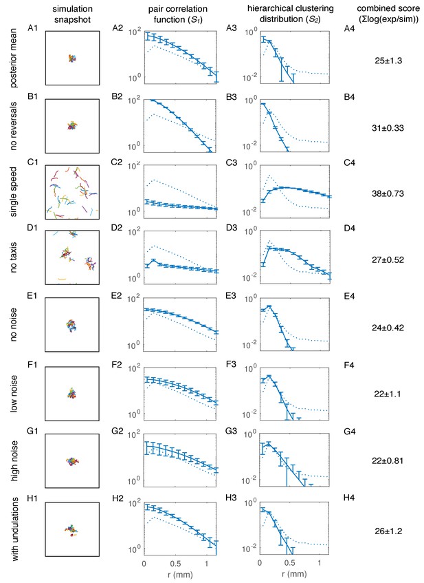
Core model components, but not noise and undulations in movement, are necessary for quantitative agreement with aggregation summary statistics.
(A) Simulation for parameters equal to the mean of the posterior distribution for the npr-1 strain (Figure 6C). (A1), Sample snapshot of simulation; (A2), Pair correlation statistic, averaged over ten simulations (solid line), and standard error of the mean (error bars), with experimental reference (dotted line, as in Figure 6B); (A3), Hierarchical clustering distribution, averaged over ten simulations (solid line), and standard error of the mean (error bars), with experimental reference (dotted line, as in Figure 6B); (A4), Combined score for model agreement with experiment (lower score is better) for summary statistics in (A1) and (A2), calculated as the difference in the logarithm of the summary statistics between experiment and simulation (see Appendix 1 for details). (B) As in (A) but with r' = 0 (no reversals). (C) As in (A) but with worms always moving at the faster speed. (D) As in (A) but with ft = 0 (no taxis towards other worms). (E) As in (A) but with η = 0 (no directional noise in movement). (F) As in (A) but with η = 0.005. This η represents directional noise 10 times lower than in (A). (G) As in (A) but with η = 0.08. This η represents higher noise than in (A), and roughly corresponds to the velocity autocorrelation measured for interacting worms in our experiments (Figure 6 – figure supplement 4A2-3). (H) As in (A) but with sinusoidal undulations in the direction of movement, with a frequency similar to that of npr-1 worms (see Appendix 1 for details).
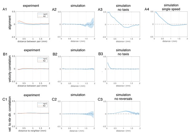
Analysis of orientational and velocity correlations in experiments and simulations.
(A) Orientational correlation quantifies the alignment of the pharynxes (experiments, (A1), or first three nodes (simulations, A2-4) between pairs of worms a given distance apart. A value of 1 corresponds to parallel alignment, and −1 to anti-parallel alignment. Solid lines show the average directional correlation and shaded area shows the 95% confidence interval. (A1), Experimental measurements; (A2), Simulation for parameters equal to mean of posterior distribution for npr-1 strain (Figure 6C); (A3), As in (A2) but with ft = 0 (no taxis towards other worms); (A4), As in (A2) but with worms always moving at the faster speed. (B) Velocity correlation quantifies the alignment of movement directions between pairs of worms a given distance apart. A value of 1 corresponds to worms moving in the same direction, and −1 to worms moving in opposite directions. Solid lines show the average directional correlation and shaded area shows the 95% confidence interval. (B1), Experimental measurements; (B2), Simulation for parameters equal to the mean of the posterior distribution for the npr-1 strain (Figure 6C); (B3), As in (B2) but with ft = 0 (no taxis towards other worms). (C) Correlation between velocity of a worm and the direction to each neighbor was calculated to quantify the degree of taxis towards other worms. A value of 1 corresponds to worms moving directly towards a neighbor, and −1 to directly moving away from a neighbor. Solid lines show the average directional correlation and shaded area shows the 95% confidence interval. (C1), Experimental measurements; (C2), Simulation for parameters equal to the mean of the posterior distribution for npr-1 strain (Figure 6C); (C3), As in (C2) but with r' = 0 (no reversals).
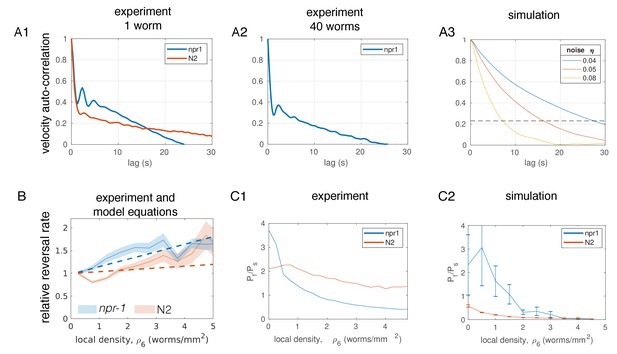
Additional comparison of model parameters with experimental measurements.
(A) Velocity autocorrelation. (A1), From experiments with body wall muscle-tracked single worms on circular food patches; (A2), From experiments with 40 worms, of which a few were body wall muscle-tracked to allow acquisition of longer trajectories; (A3), From simulated, non-interacting worms undergoing a persistent random walk for different parameter values of η, the strength of the angular noise. The dashed line shows a value of 0.23, corresponding approximately to the expected correlation for choosing angles at random, uniformly distributed between −3/4π and 3/4π, thus representing an almost complete reorientation with respect to the original direction of motion. Note that this level is reached after about 15 s for η = 0.05 and for single worms (A1), and after about 8 s for η = 0.08 and interacting worms (A2). (B) Relative reversal rates at various local densities from experiments (solid lines and shaded 95% confidence interval, same data as in Figure 3B) and from model equations for reversal rates, parameterized with the mean of posterior distribution (dotted lines). (C) Speed switching rates at various local densities. (C1), Ratio of worms moving at fast (up to 350 μm/s) versus slow (<100 μm/s for npr-1,<50 μm/s for N2) speeds as measured in experiments; (C2), Ratio of worms moving at fast versus slow (<100 μm/s for npr-1,<50 μm/s for N2) speeds as measured in simulations with posterior mean parameters, showing average over ten (npr-1) and eight (N2) simulations, error bars showing error in the mean. The disagreement may indicate that the exponential form of kf(ρ) (see Figure 5C and main text) is only a rough estimate. For (B) and (CC), inferred model parameters were converted to units of worms/mm2.
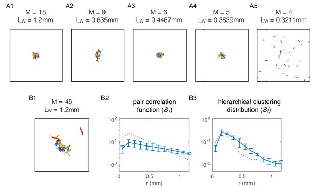
Aggregation model requires minimum length of simulated worms, and is robust to introducing volume exclusion.
(A) Simulations with decreasing length of agents. (A1), Snapshot of simulation with posterior mean parameter values for npr-1, as in Figure 6—figure supplement 2A. Worms have M = 18 nodes and a total length of Lw = 1.2 mm; (A2), Modified model with M = 9 nodes and shorter worms (but same width) still produces aggregation, without readjusting other parameters; (A3), As in (A2) but with M = 6 nodes per worm and shorter total length; (A4), As in (A2) but with M = 5 nodes per worm and shorter total length; (A5), at M = 4 nodes per worm and corresponding length of Lw = 0.3211 mm, stable aggregates comprising all worms fail to form. At this worm length, the interaction radii of head and tail nodes start to overlap, and worms require a difference in contact between head and tail to initiate reversals in our simulations. (B) Simulations with volume exclusion. (B1), Snapshot of simulation where volume exclusion is enforced, such that worms cannot overlap (apart from themselves), without adjusting any other parameters. The number of nodes per worm has been increased to M = 45 to ensure sufficient overlap between nodes within a worm. Pair correlation function (B2) and hierarchical clustering distribution (B3) show that aggregate is spread out and less dense compared to experiments (dotted line). Solid lines show mean over three simulations and error bars show standard deviation.
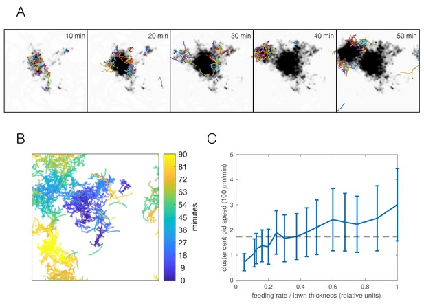
Simulations capture dynamic swarming.
(A) Snapshots of aggregation simulation with food depletion. Background color shows relative food concentration with white indicating high food and black indicating no food. (B) Visualization of worm positions in (A) over time, showing cluster displacement. Note the periodic boundary conditions. (C) Cluster speed at various feeding rates relative to lawn thickness (other parameters equal to mean of posterior distribution for npr-1). The upward trend is expected: smaller lawn thickness leads to faster movement as worms run out of food quicker and need to re-form clusters on nearby food. Cluster speed is calculated the same way as in Figure 1D; error bars show median absolute deviation over five simulations. Dashed line indicates experimentally-derived median cluster speed (from Figure 1D) for comparison.
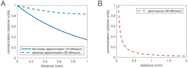
Oxygen consumption-diffusion calculations predict shallow O2 concentration gradients.
(A) Plot of feasible oxygen gradients inside worm aggregates. The oxygen concentration decays with length constant , with diffusion constant (in water) and oxygen consumption rate (estimated as an upper bound for 200 pl/min [Shoyama et al., 2009; Suda et al., 2005] at 21% oxygen and 8000 pl worm volume). The thinnest dimension of a cluster is relevant for diffusion, which is its thickness. We can approximate the cluster geometry either as flat, which results in a 1D diffusion gradient (solid line), or as hemispherical, which we approximate by spherically symmetric diffusion in 3D (dashed line). In either case the reaction-diffusion equation was solved at steady state. (B) Gradient of diffusible, non-degrading signal, ∂t for example CO2, outside a point source. Without decay, this problem is equivalent to calculating the λ potential around a point charge, and the concentration would be , in 3D, where λ is the production rate times the volume of a worm, 0.14/min (equal and opposite to the O2 consumption, based on mass conservation). A point source represents the contribution of a short section of a worm, and the contributions of many worms in an aggregate would integrate to give an approximately logarithmic gradient of signal outside the aggregate.
Videos
Sample video showing npr-1 collective feeding dynamics (bright field high-number swarming imaging).
The video plays at 300x the normal speed.
Sample video showing npr-1 collective feeding dynamics (fluorescence 40 worm aggregation imaging).
The video plays at 90x the normal speed.
A single event showing switch from high to low motility state prior to cluster entry (fluorescence 40 worm aggregation imaging).
The red worm at the bottom (arrow) decreases speed before entering a cluster. Inset: midbody absolute speed of that individual with respect to time 0 as the point of the head entering a cluster; open blue circle shows the current speed matched to the video frame.
A single event showing switch from low to high motility state prior to cluster exit (fluorescence 40 worm aggregation imaging).
The red worm increases speed before exiting a cluster. Inset: midbody absolute speed of that individual with respect to time 0 as the point of the head exiting a cluster; open blue circle shows the current speed matched to the video frame.
Sample model (with taxis) simulation describing npr-1 mutants.
The video plays at 30x the normal speed.
Sample model (with taxis) simulation describing N2.
The video plays at 30x the normal speed.
Sample swarming simulation describing npr-1 mutants.
Background color shows relative food concentration with white indicating high food and black indicating no food.The video plays at 30x the normal speed.
Tables
| Resource | Designation | Source or reference | Identifiers | Additional information |
|---|---|---|---|---|
| Strain (C. elegans) | N2 | Caenorhabditis Genetics Centre | RRID:WB-STRAIN:N2 | Laboratory reference strain. |
| Strain (C. elegans) | DA609 | Caenorhabditis Genetics Centre | RRID:WB-STRAIN:DA609 | Genotype: npr-1(ad609)X. |
| Strain (C. elegans) | OMG2 | this paper | Genotype: mIs12[myo-2p::GFP]II; npr-1(ad609)X. Originated from CB5584 and DA609. | |
| Strain (C. elegans) | OMG10 | this paper | Genotype: mIs12[myo-2p::GFP]II. Originated from CB5584; outcrossed 6x to CGC N2. | |
| Strain (C. elegans) | OMG19 | this paper | Genotype: rmIs349[myo3p::RFP]; npr-1(ad609)X. Originated from AM1065 and DA609. | |
| Strain (C. elegans) | OMG24 | this paper | Genotype: rmIs349[myo3p::RFP]. Originated from AM1065; outcrossed 6x to CGC N2. | |
| Strain (C. elegans) | DR476 | Caenorhabditis Genetics Centre | RRID:WB-STRAIN:DR476 | Genotype: daf-22(m130)II. |
| Strain (C. elegans) | AX994 | Mario de Bono (MRC Laboratory of Molecular Biology) | Genotype: daf-22(m130)II; npr-1(ad609)X. | |
| Software | Tierpsy Tracker (v 1.3) | Javer et al., 2018 | Software available at ver228. github.io/tierpsy-tracker. | |
| Software | wormTrackingAnalysis | this paper | Software available at github.com/ljschumacher/wormTrackingAnalysis. | |
| Software | sworm-model | this paper | Software available at github.com/ljschumacher/sworm-model. |
Additional files
-
Supplementary file 1
Model parameters.
- https://doi.org/10.7554/eLife.43318.026
-
Supplementary file 2
Imaging datasets used in this study.
- https://doi.org/10.7554/eLife.43318.027
-
Transparent reporting form
- https://doi.org/10.7554/eLife.43318.028


